Loading and Visualization#
In this section, we illustrate how to load and visualize the pseudoPAGES2k dataset with cfr.
Required data to complete this tutorial:
pseudoPAGES2k: ppwn_SNRinf_rta.nc
[1]:
%load_ext autoreload
%autoreload 2

import cfr
print(cfr.__version__)
import xarray as xr
2023.7.21
Load the pseudoPAGES2k dataset with xarray#
By default, we may load a netCDF file with xarray to have a check of the data structure:
[2]:
ds = xr.open_dataset('./data/ppwn_SNRinf_rta.nc', use_cftime=True)
ds
[2]:
<xarray.Dataset>
Dimensions:  (time: 1156)
Coordinates:
  * time     (time) object 0850-01-01 00:00:00 ... 2005-01-01 00:00:00
Data variables: (12/558)
    NAm_153  (time) float64 ...
    NAm_165  (time) float64 ...
    Asi_178  (time) float64 ...
    Asi_174  (time) float64 ...
    Asi_198  (time) float64 ...
    NAm_145  (time) float64 ...
    ...       ...
    Ocn_169  (time) float64 ...
    Asi_201  (time) float64 ...
    Asi_179  (time) float64 ...
    Arc_014  (time) float64 ...
    Ocn_071  (time) float64 ...
Ocn_072 (time) float64 ...- time: 1156
- time(time)object0850-01-01 00:00:00 ... 2005-01-...
array([cftime.DatetimeGregorian(850, 1, 1, 0, 0, 0, 0, has_year_zero=False),
       cftime.DatetimeGregorian(851, 1, 1, 0, 0, 0, 0, has_year_zero=False),
       cftime.DatetimeGregorian(852, 1, 1, 0, 0, 0, 0, has_year_zero=False),
       ...,
       cftime.DatetimeGregorian(2003, 1, 1, 0, 0, 0, 0, has_year_zero=False),
       cftime.DatetimeGregorian(2004, 1, 1, 0, 0, 0, 0, has_year_zero=False),
       cftime.DatetimeGregorian(2005, 1, 1, 0, 0, 0, 0, has_year_zero=False)],
      dtype=object)
- NAm_153(time)float64...
- lat :
- 52.7
- lon :
- 241.7
- elev :
- nan
- ptype :
- tree.TRW
- dt :
- 1.0
- time_name :
- Time
- time_unit :
- yr
- value_name :
- trsgi
- value_unit :
- NA
[1156 values with dtype=float64]
- NAm_165(time)float64...
- lat :
- 37.9
- lon :
- 252.3
- elev :
- nan
- ptype :
- tree.MXD
- dt :
- 1.0
- time_name :
- Time
- time_unit :
- yr
- value_name :
- MXD
- value_unit :
- NA
[1156 values with dtype=float64]
- Asi_178(time)float64...
- lat :
- 28.77
- lon :
- 83.73
- elev :
- nan
- ptype :
- tree.TRW
- dt :
- 1.0
- time_name :
- Time
- time_unit :
- yr
- value_name :
- trsgi
- value_unit :
- NA
[1156 values with dtype=float64]
- Asi_174(time)float64...
- lat :
- 28.18
- lon :
- 85.43
- elev :
- nan
- ptype :
- tree.TRW
- dt :
- 1.0
- time_name :
- Time
- time_unit :
- yr
- value_name :
- trsgi
- value_unit :
- NA
[1156 values with dtype=float64]
- Asi_198(time)float64...
- lat :
- 35.35
- lon :
- 71.93
- elev :
- nan
- ptype :
- tree.TRW
- dt :
- 1.0
- time_name :
- Time
- time_unit :
- yr
- value_name :
- trsgi
- value_unit :
- NA
[1156 values with dtype=float64]
- NAm_145(time)float64...
- lat :
- 59.9
- lon :
- 223.2
- elev :
- nan
- ptype :
- tree.TRW
- dt :
- 1.0
- time_name :
- Time
- time_unit :
- yr
- value_name :
- trsgi
- value_unit :
- NA
[1156 values with dtype=float64]
- Arc_071(time)float64...
- lat :
- 68.49166667
- lon :
- 27.33333333
- elev :
- nan
- ptype :
- tree.MXD
- dt :
- 1.0
- time_name :
- Time
- time_unit :
- yr
- value_name :
- MXD
- value_unit :
- NaN
[1156 values with dtype=float64]
- NAm_102(time)float64...
- lat :
- 62.0
- lon :
- 218.0
- elev :
- nan
- ptype :
- tree.MXD
- dt :
- 1.0
- time_name :
- Time
- time_unit :
- yr
- value_name :
- MXD
- value_unit :
- NA
[1156 values with dtype=float64]
- NAm_046(time)float64...
- lat :
- 46.0
- lon :
- 246.6
- elev :
- nan
- ptype :
- tree.TRW
- dt :
- 1.0
- time_name :
- Time
- time_unit :
- yr
- value_name :
- trsgi
- value_unit :
- NA
[1156 values with dtype=float64]
- Asi_170(time)float64...
- lat :
- 28.38
- lon :
- 83.7
- elev :
- nan
- ptype :
- tree.TRW
- dt :
- 1.0
- time_name :
- Time
- time_unit :
- yr
- value_name :
- trsgi
- value_unit :
- NA
[1156 values with dtype=float64]
- Ant_023(time)float64...
- lat :
- -77.78
- lon :
- 158.72
- elev :
- nan
- ptype :
- ice.d18O
- dt :
- 1.0
- time_name :
- Time
- time_unit :
- yr
- value_name :
- d18O
- value_unit :
- permil
[1156 values with dtype=float64]
- Asi_045(time)float64...
- lat :
- 34.73
- lon :
- 100.78
- elev :
- nan
- ptype :
- tree.TRW
- dt :
- 1.0
- time_name :
- Time
- time_unit :
- yr
- value_name :
- trsgi
- value_unit :
- NA
[1156 values with dtype=float64]
- NAm_149(time)float64...
- lat :
- 60.1
- lon :
- 225.6
- elev :
- nan
- ptype :
- tree.TRW
- dt :
- 1.0
- time_name :
- Time
- time_unit :
- yr
- value_name :
- trsgi
- value_unit :
- NA
[1156 values with dtype=float64]
- NAm_193(time)float64...
- lat :
- 48.7
- lon :
- 241.7
- elev :
- nan
- ptype :
- tree.TRW
- dt :
- 1.0
- time_name :
- Time
- time_unit :
- yr
- value_name :
- trsgi
- value_unit :
- NA
[1156 values with dtype=float64]
- NAm_194(time)float64...
- lat :
- 48.7
- lon :
- 241.7
- elev :
- nan
- ptype :
- tree.MXD
- dt :
- 1.0
- time_name :
- Time
- time_unit :
- yr
- value_name :
- MXD
- value_unit :
- NA
[1156 values with dtype=float64]
- NAm_089(time)float64...
- lat :
- 63.3
- lon :
- 212.2
- elev :
- nan
- ptype :
- tree.TRW
- dt :
- 1.0
- time_name :
- Time
- time_unit :
- yr
- value_name :
- trsgi
- value_unit :
- NA
[1156 values with dtype=float64]
- NAm_188(time)float64...
- lat :
- 49.8
- lon :
- 245.5
- elev :
- nan
- ptype :
- tree.TRW
- dt :
- 1.0
- time_name :
- Time
- time_unit :
- yr
- value_name :
- trsgi
- value_unit :
- NA
[1156 values with dtype=float64]
- Asi_184(time)float64...
- lat :
- 35.33
- lon :
- 74.8
- elev :
- nan
- ptype :
- tree.TRW
- dt :
- 1.0
- time_name :
- Time
- time_unit :
- yr
- value_name :
- trsgi
- value_unit :
- NA
[1156 values with dtype=float64]
- Asi_214(time)float64...
- lat :
- 35.35
- lon :
- 71.8
- elev :
- nan
- ptype :
- tree.TRW
- dt :
- 1.0
- time_name :
- Time
- time_unit :
- yr
- value_name :
- trsgi
- value_unit :
- NA
[1156 values with dtype=float64]
- Ocn_075(time)float64...
- lat :
- -23.15
- lon :
- 43.58
- elev :
- nan
- ptype :
- coral.d18O
- dt :
- 1.0
- time_name :
- Time
- time_unit :
- yr
- value_name :
- d18O
- value_unit :
- permil
[1156 values with dtype=float64]
- Asi_147(time)float64...
- lat :
- 49.92
- lon :
- 91.57
- elev :
- nan
- ptype :
- tree.TRW
- dt :
- 1.0
- time_name :
- Time
- time_unit :
- yr
- value_name :
- trsgi
- value_unit :
- NA
[1156 values with dtype=float64]
- Asi_098(time)float64...
- lat :
- 36.68
- lon :
- 98.42
- elev :
- nan
- ptype :
- tree.TRW
- dt :
- 1.0
- time_name :
- Time
- time_unit :
- yr
- value_name :
- trsgi
- value_unit :
- NA
[1156 values with dtype=float64]
- NAm_099(time)float64...
- lat :
- 56.0
- lon :
- 228.0
- elev :
- nan
- ptype :
- tree.TRW
- dt :
- 1.0
- time_name :
- Time
- time_unit :
- yr
- value_name :
- trsgi
- value_unit :
- NA
[1156 values with dtype=float64]
- Asi_070(time)float64...
- lat :
- 28.9
- lon :
- 99.75
- elev :
- nan
- ptype :
- tree.TRW
- dt :
- 1.0
- time_name :
- Time
- time_unit :
- yr
- value_name :
- trsgi
- value_unit :
- NA
[1156 values with dtype=float64]
- Asi_215(time)float64...
- lat :
- 35.88
- lon :
- 74.88
- elev :
- nan
- ptype :
- tree.TRW
- dt :
- 1.0
- time_name :
- Time
- time_unit :
- yr
- value_name :
- trsgi
- value_unit :
- NA
[1156 values with dtype=float64]
- Asi_223(time)float64...
- lat :
- 29.62
- lon :
- 94.67
- elev :
- nan
- ptype :
- tree.TRW
- dt :
- 1.0
- time_name :
- Time
- time_unit :
- yr
- value_name :
- trsgi
- value_unit :
- NA
[1156 values with dtype=float64]
- NAm_156(time)float64...
- lat :
- 52.6
- lon :
- 242.1
- elev :
- nan
- ptype :
- tree.TRW
- dt :
- 1.0
- time_name :
- Time
- time_unit :
- yr
- value_name :
- trsgi
- value_unit :
- NA
[1156 values with dtype=float64]
- Asi_009(time)float64...
- lat :
- 50.48
- lon :
- 87.67
- elev :
- nan
- ptype :
- tree.TRW
- dt :
- 1.0
- time_name :
- Time
- time_unit :
- yr
- value_name :
- trsgi
- value_unit :
- NA
[1156 values with dtype=float64]
- Asi_173(time)float64...
- lat :
- 29.52
- lon :
- 82.03
- elev :
- nan
- ptype :
- tree.TRW
- dt :
- 1.0
- time_name :
- Time
- time_unit :
- yr
- value_name :
- trsgi
- value_unit :
- NA
[1156 values with dtype=float64]
- Asi_047(time)float64...
- lat :
- 37.93
- lon :
- 101.53
- elev :
- nan
- ptype :
- tree.TRW
- dt :
- 1.0
- time_name :
- Time
- time_unit :
- yr
- value_name :
- trsgi
- value_unit :
- NA
[1156 values with dtype=float64]
- Ocn_078(time)float64...
- lat :
- -3.2
- lon :
- 40.1
- elev :
- nan
- ptype :
- coral.d18O
- dt :
- 1.0
- time_name :
- Time
- time_unit :
- yr
- value_name :
- d18O
- value_unit :
- permil
[1156 values with dtype=float64]
- NAm_154(time)float64...
- lat :
- 51.7
- lon :
- 243.5
- elev :
- nan
- ptype :
- tree.TRW
- dt :
- 1.0
- time_name :
- Time
- time_unit :
- yr
- value_name :
- trsgi
- value_unit :
- NA
[1156 values with dtype=float64]
- Asi_148(time)float64...
- lat :
- 48.17
- lon :
- 99.87
- elev :
- nan
- ptype :
- tree.TRW
- dt :
- 1.0
- time_name :
- Time
- time_unit :
- yr
- value_name :
- trsgi
- value_unit :
- NA
[1156 values with dtype=float64]
- Asi_191(time)float64...
- lat :
- 35.68
- lon :
- 71.63
- elev :
- nan
- ptype :
- tree.TRW
- dt :
- 1.0
- time_name :
- Time
- time_unit :
- yr
- value_name :
- trsgi
- value_unit :
- NA
[1156 values with dtype=float64]
- Asi_062(time)float64...
- lat :
- 34.48
- lon :
- 110.08
- elev :
- nan
- ptype :
- tree.TRW
- dt :
- 1.0
- time_name :
- Time
- time_unit :
- yr
- value_name :
- trsgi
- value_unit :
- NA
[1156 values with dtype=float64]
- Asi_019(time)float64...
- lat :
- 50.15
- lon :
- 85.37
- elev :
- nan
- ptype :
- tree.TRW
- dt :
- 1.0
- time_name :
- Time
- time_unit :
- yr
- value_name :
- trsgi
- value_unit :
- NA
[1156 values with dtype=float64]
- Ocn_167(time)float64...
- lat :
- 16.85
- lon :
- 112.33
- elev :
- nan
- ptype :
- coral.SrCa
- dt :
- 1.0
- time_name :
- Time
- time_unit :
- yr
- value_name :
- Sr_Ca
- value_unit :
- mmol/mol
[1156 values with dtype=float64]
- NAm_085(time)float64...
- lat :
- 61.8
- lon :
- 212.7
- elev :
- nan
- ptype :
- tree.TRW
- dt :
- 1.0
- time_name :
- Time
- time_unit :
- yr
- value_name :
- trsgi
- value_unit :
- NA
[1156 values with dtype=float64]
- NAm_086(time)float64...
- lat :
- 61.8
- lon :
- 212.7
- elev :
- nan
- ptype :
- tree.MXD
- dt :
- 1.0
- time_name :
- Time
- time_unit :
- yr
- value_name :
- MXD
- value_unit :
- NA
[1156 values with dtype=float64]
- Ocn_091(time)float64...
- lat :
- -16.8167
- lon :
- 179.2333
- elev :
- nan
- ptype :
- coral.d18O
- dt :
- 1.0
- time_name :
- Time
- time_unit :
- yr
- value_name :
- d18O
- value_unit :
- permil
[1156 values with dtype=float64]
- Ocn_093(time)float64...
- lat :
- -16.8167
- lon :
- 179.2333
- elev :
- nan
- ptype :
- coral.SrCa
- dt :
- 1.0
- time_name :
- Time
- time_unit :
- yr
- value_name :
- Sr_Ca
- value_unit :
- mmol/mol
[1156 values with dtype=float64]
- Asi_155(time)float64...
- lat :
- 48.3
- lon :
- 98.93
- elev :
- nan
- ptype :
- tree.TRW
- dt :
- 1.0
- time_name :
- Time
- time_unit :
- yr
- value_name :
- trsgi
- value_unit :
- NA
[1156 values with dtype=float64]
- Ant_024(time)float64...
- lat :
- -86.5
- lon :
- 252.01
- elev :
- nan
- ptype :
- ice.d18O
- dt :
- 1.0
- time_name :
- Time
- time_unit :
- yr
- value_name :
- d18O
- value_unit :
- permil
[1156 values with dtype=float64]
- NAm_098(time)float64...
- lat :
- 58.4
- lon :
- 225.4
- elev :
- nan
- ptype :
- tree.TRW
- dt :
- 1.0
- time_name :
- Time
- time_unit :
- yr
- value_name :
- trsgi
- value_unit :
- NA
[1156 values with dtype=float64]
- Asi_073(time)float64...
- lat :
- 27.33
- lon :
- 99.3
- elev :
- nan
- ptype :
- tree.TRW
- dt :
- 1.0
- time_name :
- Time
- time_unit :
- yr
- value_name :
- trsgi
- value_unit :
- NA
[1156 values with dtype=float64]
- Asi_209(time)float64...
- lat :
- 36.15
- lon :
- 74.18
- elev :
- nan
- ptype :
- tree.TRW
- dt :
- 1.0
- time_name :
- Time
- time_unit :
- yr
- value_name :
- trsgi
- value_unit :
- NA
[1156 values with dtype=float64]
- Asi_094(time)float64...
- lat :
- 37.32
- lon :
- 98.4
- elev :
- nan
- ptype :
- tree.TRW
- dt :
- 1.0
- time_name :
- Time
- time_unit :
- yr
- value_name :
- trsgi
- value_unit :
- NA
[1156 values with dtype=float64]
- Arc_001(time)float64...
- lat :
- 68.09
- lon :
- 209.53
- elev :
- nan
- ptype :
- lake.varve_thickness
- dt :
- 1.0
- time_name :
- Time
- time_unit :
- yr
- value_name :
- thickness
- value_unit :
- cm
[1156 values with dtype=float64]
- Ocn_096(time)float64...
- lat :
- -21.2378
- lon :
- 200.1722
- elev :
- nan
- ptype :
- coral.SrCa
- dt :
- 1.0
- time_name :
- Time
- time_unit :
- yr
- value_name :
- Sr_Ca
- value_unit :
- mmol/mol
[1156 values with dtype=float64]
- Asi_052(time)float64...
- lat :
- 34.78
- lon :
- 99.78
- elev :
- nan
- ptype :
- tree.TRW
- dt :
- 1.0
- time_name :
- Time
- time_unit :
- yr
- value_name :
- trsgi
- value_unit :
- NA
[1156 values with dtype=float64]
- Ocn_086(time)float64...
- lat :
- -1.5
- lon :
- 124.833
- elev :
- nan
- ptype :
- coral.d18O
- dt :
- 1.0
- time_name :
- Time
- time_unit :
- yr
- value_name :
- d18O
- value_unit :
- permil
[1156 values with dtype=float64]
- NAm_122(time)float64...
- lat :
- 51.8
- lon :
- 243.8
- elev :
- nan
- ptype :
- tree.MXD
- dt :
- 1.0
- time_name :
- Time
- time_unit :
- yr
- value_name :
- MXD
- value_unit :
- NA
[1156 values with dtype=float64]
- Asi_150(time)float64...
- lat :
- 48.7
- lon :
- 88.8
- elev :
- nan
- ptype :
- tree.TRW
- dt :
- 1.0
- time_name :
- Time
- time_unit :
- yr
- value_name :
- trsgi
- value_unit :
- NA
[1156 values with dtype=float64]
- Asi_117(time)float64...
- lat :
- 30.37
- lon :
- 130.53
- elev :
- nan
- ptype :
- tree.TRW
- dt :
- 1.0
- time_name :
- Time
- time_unit :
- yr
- value_name :
- trsgi
- value_unit :
- NA
[1156 values with dtype=float64]
- NAm_186(time)float64...
- lat :
- 49.3
- lon :
- 245.6
- elev :
- nan
- ptype :
- tree.TRW
- dt :
- 1.0
- time_name :
- Time
- time_unit :
- yr
- value_name :
- trsgi
- value_unit :
- NA
[1156 values with dtype=float64]
- NAm_161(time)float64...
- lat :
- 52.9
- lon :
- 242.0
- elev :
- nan
- ptype :
- tree.TRW
- dt :
- 1.0
- time_name :
- Time
- time_unit :
- yr
- value_name :
- trsgi
- value_unit :
- NA
[1156 values with dtype=float64]
- Asi_030(time)float64...
- lat :
- 27.63
- lon :
- 90.13
- elev :
- nan
- ptype :
- tree.TRW
- dt :
- 1.0
- time_name :
- Time
- time_unit :
- yr
- value_name :
- trsgi
- value_unit :
- NA
[1156 values with dtype=float64]
- Ocn_101(time)float64...
- lat :
- -22.475
- lon :
- 166.4667
- elev :
- nan
- ptype :
- coral.SrCa
- dt :
- 1.0
- time_name :
- Time
- time_unit :
- yr
- value_name :
- Sr_Ca
- value_unit :
- mmol/mol
[1156 values with dtype=float64]
- NAm_066(time)float64...
- lat :
- 46.7
- lon :
- 245.8
- elev :
- nan
- ptype :
- tree.TRW
- dt :
- 1.0
- time_name :
- Time
- time_unit :
- yr
- value_name :
- trsgi
- value_unit :
- NA
[1156 values with dtype=float64]
- Asi_108(time)float64...
- lat :
- 43.77
- lon :
- 142.55
- elev :
- nan
- ptype :
- tree.TRW
- dt :
- 1.0
- time_name :
- Time
- time_unit :
- yr
- value_name :
- trsgi
- value_unit :
- NA
[1156 values with dtype=float64]
- Ocn_070(time)float64...
- lat :
- 24.6
- lon :
- 277.7
- elev :
- nan
- ptype :
- coral.SrCa
- dt :
- 1.0
- time_name :
- Time
- time_unit :
- yr
- value_name :
- Sr_Ca
- value_unit :
- mmol/mol
[1156 values with dtype=float64]
- Asi_084(time)float64...
- lat :
- 37.47
- lon :
- 97.23
- elev :
- nan
- ptype :
- tree.TRW
- dt :
- 1.0
- time_name :
- Time
- time_unit :
- yr
- value_name :
- trsgi
- value_unit :
- NA
[1156 values with dtype=float64]
- Ocn_076(time)float64...
- lat :
- -3.2
- lon :
- 40.1
- elev :
- nan
- ptype :
- coral.d18O
- dt :
- 1.0
- time_name :
- Time
- time_unit :
- yr
- value_name :
- d18O
- value_unit :
- permil
[1156 values with dtype=float64]
- NAm_050(time)float64...
- lat :
- 38.5
- lon :
- 245.8
- elev :
- nan
- ptype :
- tree.TRW
- dt :
- 1.0
- time_name :
- Time
- time_unit :
- yr
- value_name :
- trsgi
- value_unit :
- NA
[1156 values with dtype=float64]
- Asi_135(time)float64...
- lat :
- 42.2
- lon :
- 79.05
- elev :
- nan
- ptype :
- tree.TRW
- dt :
- 1.0
- time_name :
- Time
- time_unit :
- yr
- value_name :
- trsgi
- value_unit :
- NA
[1156 values with dtype=float64]
- Asi_144(time)float64...
- lat :
- 48.27
- lon :
- 88.87
- elev :
- nan
- ptype :
- tree.TRW
- dt :
- 1.0
- time_name :
- Time
- time_unit :
- yr
- value_name :
- trsgi
- value_unit :
- NA
[1156 values with dtype=float64]
- Asi_185(time)float64...
- lat :
- 35.33
- lon :
- 74.8
- elev :
- nan
- ptype :
- tree.TRW
- dt :
- 1.0
- time_name :
- Time
- time_unit :
- yr
- value_name :
- trsgi
- value_unit :
- NA
[1156 values with dtype=float64]
- Asi_029(time)float64...
- lat :
- 27.67
- lon :
- 90.72
- elev :
- nan
- ptype :
- tree.TRW
- dt :
- 1.0
- time_name :
- Time
- time_unit :
- yr
- value_name :
- trsgi
- value_unit :
- NA
[1156 values with dtype=float64]
- Asi_115(time)float64...
- lat :
- 43.5
- lon :
- 143.2
- elev :
- nan
- ptype :
- tree.TRW
- dt :
- 1.0
- time_name :
- Time
- time_unit :
- yr
- value_name :
- trsgi
- value_unit :
- NA
[1156 values with dtype=float64]
- NAm_133(time)float64...
- lat :
- 50.2
- lon :
- 242.9
- elev :
- nan
- ptype :
- tree.TRW
- dt :
- 1.0
- time_name :
- Time
- time_unit :
- yr
- value_name :
- trsgi
- value_unit :
- NA
[1156 values with dtype=float64]
- NAm_134(time)float64...
- lat :
- 50.2
- lon :
- 242.9
- elev :
- nan
- ptype :
- tree.MXD
- dt :
- 1.0
- time_name :
- Time
- time_unit :
- yr
- value_name :
- MXD
- value_unit :
- NA
[1156 values with dtype=float64]
- Asi_243(time)float64...
- lat :
- 33.9167
- lon :
- 89.0833
- elev :
- nan
- ptype :
- ice.d18O
- dt :
- 1.0
- time_name :
- Time
- time_unit :
- yr
- value_name :
- d18O
- value_unit :
- permil
[1156 values with dtype=float64]
- Asi_146(time)float64...
- lat :
- 49.37
- lon :
- 94.88
- elev :
- nan
- ptype :
- tree.TRW
- dt :
- 1.0
- time_name :
- Time
- time_unit :
- yr
- value_name :
- trsgi
- value_unit :
- NA
[1156 values with dtype=float64]
- NAm_123(time)float64...
- lat :
- 49.4
- lon :
- 236.9
- elev :
- nan
- ptype :
- tree.MXD
- dt :
- 1.0
- time_name :
- Time
- time_unit :
- yr
- value_name :
- MXD
- value_unit :
- NA
[1156 values with dtype=float64]
- Ant_012(time)float64...
- lat :
- -79.57
- lon :
- 314.28
- elev :
- nan
- ptype :
- ice.d18O
- dt :
- 1.0
- time_name :
- Time
- time_unit :
- yr
- value_name :
- d18O
- value_unit :
- permil
[1156 values with dtype=float64]
- Asi_176(time)float64...
- lat :
- 27.67
- lon :
- 87.2
- elev :
- nan
- ptype :
- tree.TRW
- dt :
- 1.0
- time_name :
- Time
- time_unit :
- yr
- value_name :
- trsgi
- value_unit :
- NA
[1156 values with dtype=float64]
- NAm_093(time)float64...
- lat :
- 65.2
- lon :
- 197.8
- elev :
- nan
- ptype :
- tree.TRW
- dt :
- 1.0
- time_name :
- Time
- time_unit :
- yr
- value_name :
- trsgi
- value_unit :
- NA
[1156 values with dtype=float64]
- Ocn_099(time)float64...
- lat :
- -17.5
- lon :
- 210.1667
- elev :
- nan
- ptype :
- coral.d18O
- dt :
- 1.0
- time_name :
- Time
- time_unit :
- yr
- value_name :
- d18O
- value_unit :
- permil
[1156 values with dtype=float64]
- Asi_128(time)float64...
- lat :
- 40.17
- lon :
- 72.62
- elev :
- nan
- ptype :
- tree.TRW
- dt :
- 1.0
- time_name :
- Time
- time_unit :
- yr
- value_name :
- trsgi
- value_unit :
- NA
[1156 values with dtype=float64]
- Asi_228(time)float64...
- lat :
- 21.67
- lon :
- 104.1
- elev :
- nan
- ptype :
- tree.TRW
- dt :
- 1.0
- time_name :
- Time
- time_unit :
- yr
- value_name :
- trsgi
- value_unit :
- NA
[1156 values with dtype=float64]
- Ant_020(time)float64...
- lat :
- -75.58
- lon :
- 356.57
- elev :
- nan
- ptype :
- ice.d18O
- dt :
- 1.0
- time_name :
- Time
- time_unit :
- yr
- value_name :
- d18O
- value_unit :
- permil
[1156 values with dtype=float64]
- NAm_090(time)float64...
- lat :
- 65.2
- lon :
- 197.8
- elev :
- nan
- ptype :
- tree.TRW
- dt :
- 1.0
- time_name :
- Time
- time_unit :
- yr
- value_name :
- trsgi
- value_unit :
- NA
[1156 values with dtype=float64]
- Ocn_144(time)float64...
- lat :
- 30.0867
- lon :
- 295.4583
- elev :
- nan
- ptype :
- coral.d18O
- dt :
- 1.0
- time_name :
- Time
- time_unit :
- yr
- value_name :
- d18O
- value_unit :
- permil
[1156 values with dtype=float64]
- Asi_202(time)float64...
- lat :
- 36.58
- lon :
- 75.08
- elev :
- nan
- ptype :
- tree.TRW
- dt :
- 1.0
- time_name :
- Time
- time_unit :
- yr
- value_name :
- trsgi
- value_unit :
- NA
[1156 values with dtype=float64]
- NAm_189(time)float64...
- lat :
- 48.7
- lon :
- 239.3
- elev :
- nan
- ptype :
- tree.TRW
- dt :
- 1.0
- time_name :
- Time
- time_unit :
- yr
- value_name :
- trsgi
- value_unit :
- NA
[1156 values with dtype=float64]
- NAm_171(time)float64...
- lat :
- 40.6
- lon :
- 254.2
- elev :
- nan
- ptype :
- tree.TRW
- dt :
- 1.0
- time_name :
- Time
- time_unit :
- yr
- value_name :
- trsgi
- value_unit :
- NA
[1156 values with dtype=float64]
- Ocn_178(time)float64...
- lat :
- -21.2378
- lon :
- 200.1722
- elev :
- nan
- ptype :
- coral.d18O
- dt :
- 1.0
- time_name :
- Time
- time_unit :
- yr
- value_name :
- d18O
- value_unit :
- permil
[1156 values with dtype=float64]
- Asi_203(time)float64...
- lat :
- 36.58
- lon :
- 75.08
- elev :
- nan
- ptype :
- tree.TRW
- dt :
- 1.0
- time_name :
- Time
- time_unit :
- yr
- value_name :
- trsgi
- value_unit :
- NA
[1156 values with dtype=float64]
- Arc_029(time)float64...
- lat :
- 80.0
- lon :
- 318.86
- elev :
- nan
- ptype :
- ice.d18O
- dt :
- 1.0
- time_name :
- Time
- time_unit :
- yr
- value_name :
- d18O
- value_unit :
- permil
[1156 values with dtype=float64]
- NAm_113(time)float64...
- lat :
- 62.7
- lon :
- 249.0
- elev :
- nan
- ptype :
- tree.MXD
- dt :
- 1.0
- time_name :
- Time
- time_unit :
- yr
- value_name :
- MXD
- value_unit :
- NA
[1156 values with dtype=float64]
- Asi_020(time)float64...
- lat :
- 50.15
- lon :
- 85.37
- elev :
- nan
- ptype :
- tree.TRW
- dt :
- 1.0
- time_name :
- Time
- time_unit :
- yr
- value_name :
- trsgi
- value_unit :
- NA
[1156 values with dtype=float64]
- Asi_171(time)float64...
- lat :
- 27.73
- lon :
- 86.33
- elev :
- nan
- ptype :
- tree.TRW
- dt :
- 1.0
- time_name :
- Time
- time_unit :
- yr
- value_name :
- trsgi
- value_unit :
- NA
[1156 values with dtype=float64]
- NAm_157(time)float64...
- lat :
- 50.6
- lon :
- 245.0
- elev :
- nan
- ptype :
- tree.TRW
- dt :
- 1.0
- time_name :
- Time
- time_unit :
- yr
- value_name :
- trsgi
- value_unit :
- NA
[1156 values with dtype=float64]
- NAm_124(time)float64...
- lat :
- 49.2
- lon :
- 234.8
- elev :
- nan
- ptype :
- tree.MXD
- dt :
- 1.0
- time_name :
- Time
- time_unit :
- yr
- value_name :
- MXD
- value_unit :
- NA
[1156 values with dtype=float64]
- Asi_006(time)float64...
- lat :
- 49.72
- lon :
- 87.28
- elev :
- nan
- ptype :
- tree.TRW
- dt :
- 1.0
- time_name :
- Time
- time_unit :
- yr
- value_name :
- trsgi
- value_unit :
- NA
[1156 values with dtype=float64]
- Asi_033(time)float64...
- lat :
- 27.25
- lon :
- 89.38
- elev :
- nan
- ptype :
- tree.TRW
- dt :
- 1.0
- time_name :
- Time
- time_unit :
- yr
- value_name :
- trsgi
- value_unit :
- NA
[1156 values with dtype=float64]
- Ocn_149(time)float64...
- lat :
- 18.4667
- lon :
- 282.05
- elev :
- nan
- ptype :
- coral.d18O
- dt :
- 1.0
- time_name :
- Time
- time_unit :
- yr
- value_name :
- d18O
- value_unit :
- permil
[1156 values with dtype=float64]
- Ocn_150(time)float64...
- lat :
- 18.4667
- lon :
- 282.05
- elev :
- nan
- ptype :
- coral.SrCa
- dt :
- 1.0
- time_name :
- Time
- time_unit :
- yr
- value_name :
- Sr_Ca
- value_unit :
- mmol/mol
[1156 values with dtype=float64]
- Asi_120(time)float64...
- lat :
- 33.73
- lon :
- 133.12
- elev :
- nan
- ptype :
- tree.TRW
- dt :
- 1.0
- time_name :
- Time
- time_unit :
- yr
- value_name :
- trsgi
- value_unit :
- NA
[1156 values with dtype=float64]
- Arc_035(time)float64...
- lat :
- 65.18
- lon :
- 316.17
- elev :
- nan
- ptype :
- ice.d18O
- dt :
- 1.0
- time_name :
- Time
- time_unit :
- yr
- value_name :
- d18O
- value_unit :
- permil
[1156 values with dtype=float64]
- Asi_065(time)float64...
- lat :
- 30.33
- lon :
- 119.43
- elev :
- nan
- ptype :
- tree.TRW
- dt :
- 1.0
- time_name :
- Time
- time_unit :
- yr
- value_name :
- trsgi
- value_unit :
- NA
[1156 values with dtype=float64]
- NAm_049(time)float64...
- lat :
- 40.2
- lon :
- 244.5
- elev :
- nan
- ptype :
- tree.TRW
- dt :
- 1.0
- time_name :
- Time
- time_unit :
- yr
- value_name :
- trsgi
- value_unit :
- NA
[1156 values with dtype=float64]
- NAm_091(time)float64...
- lat :
- 65.2
- lon :
- 197.8
- elev :
- nan
- ptype :
- tree.TRW
- dt :
- 1.0
- time_name :
- Time
- time_unit :
- yr
- value_name :
- trsgi
- value_unit :
- NA
[1156 values with dtype=float64]
- Ocn_177(time)float64...
- lat :
- 1.6792
- lon :
- 202.7527
- elev :
- nan
- ptype :
- coral.d18O
- dt :
- 1.0
- time_name :
- Time
- time_unit :
- yr
- value_name :
- d18O
- value_unit :
- permil
[1156 values with dtype=float64]
- Ocn_080(time)float64...
- lat :
- 27.85
- lon :
- 34.32
- elev :
- nan
- ptype :
- coral.d18O
- dt :
- 1.0
- time_name :
- Time
- time_unit :
- yr
- value_name :
- d18O
- value_unit :
- permil
[1156 values with dtype=float64]
- Asi_152(time)float64...
- lat :
- 47.77
- lon :
- 107.0
- elev :
- nan
- ptype :
- tree.TRW
- dt :
- 1.0
- time_name :
- Time
- time_unit :
- yr
- value_name :
- trsgi
- value_unit :
- NA
[1156 values with dtype=float64]
- Asi_043(time)float64...
- lat :
- 34.75
- lon :
- 100.82
- elev :
- nan
- ptype :
- tree.TRW
- dt :
- 1.0
- time_name :
- Time
- time_unit :
- yr
- value_name :
- trsgi
- value_unit :
- NA
[1156 values with dtype=float64]
- Ocn_108(time)float64...
- lat :
- -15.0
- lon :
- 166.99
- elev :
- nan
- ptype :
- coral.d18O
- dt :
- 1.0
- time_name :
- Time
- time_unit :
- yr
- value_name :
- d18O
- value_unit :
- permil
[1156 values with dtype=float64]
- Asi_028(time)float64...
- lat :
- 27.7
- lon :
- 90.68
- elev :
- nan
- ptype :
- tree.TRW
- dt :
- 1.0
- time_name :
- Time
- time_unit :
- yr
- value_name :
- trsgi
- value_unit :
- NA
[1156 values with dtype=float64]
- Asi_025(time)float64...
- lat :
- 27.58
- lon :
- 90.65
- elev :
- nan
- ptype :
- tree.TRW
- dt :
- 1.0
- time_name :
- Time
- time_unit :
- yr
- value_name :
- trsgi
- value_unit :
- NA
[1156 values with dtype=float64]
- Ocn_103(time)float64...
- lat :
- 5.87
- lon :
- 197.87
- elev :
- nan
- ptype :
- coral.d18O
- dt :
- 1.0
- time_name :
- Time
- time_unit :
- yr
- value_name :
- d18O
- value_unit :
- permil
[1156 values with dtype=float64]
- NAm_109(time)float64...
- lat :
- 37.9
- lon :
- 240.8
- elev :
- nan
- ptype :
- tree.TRW
- dt :
- 1.0
- time_name :
- Time
- time_unit :
- yr
- value_name :
- trsgi
- value_unit :
- NA
[1156 values with dtype=float64]
- Arc_079(time)float64...
- lat :
- 66.8
- lon :
- 68.0
- elev :
- nan
- ptype :
- tree.TRW
- dt :
- 1.0
- time_name :
- Time
- time_unit :
- yr
- value_name :
- temperature
- value_unit :
- degC
[1156 values with dtype=float64]
- Asi_060(time)float64...
- lat :
- 34.78
- lon :
- 100.82
- elev :
- nan
- ptype :
- tree.TRW
- dt :
- 1.0
- time_name :
- Time
- time_unit :
- yr
- value_name :
- trsgi
- value_unit :
- NA
[1156 values with dtype=float64]
- Asi_110(time)float64...
- lat :
- 43.88
- lon :
- 145.6
- elev :
- nan
- ptype :
- tree.TRW
- dt :
- 1.0
- time_name :
- Time
- time_unit :
- yr
- value_name :
- trsgi
- value_unit :
- NA
[1156 values with dtype=float64]
- Asi_007(time)float64...
- lat :
- 50.14
- lon :
- 87.72
- elev :
- nan
- ptype :
- tree.TRW
- dt :
- 1.0
- time_name :
- Time
- time_unit :
- yr
- value_name :
- trsgi
- value_unit :
- NA
[1156 values with dtype=float64]
- Asi_087(time)float64...
- lat :
- 37.43
- lon :
- 98.05
- elev :
- nan
- ptype :
- tree.TRW
- dt :
- 1.0
- time_name :
- Time
- time_unit :
- yr
- value_name :
- trsgi
- value_unit :
- NA
[1156 values with dtype=float64]
- Asi_116(time)float64...
- lat :
- 44.95
- lon :
- 142.12
- elev :
- nan
- ptype :
- tree.TRW
- dt :
- 1.0
- time_name :
- Time
- time_unit :
- yr
- value_name :
- trsgi
- value_unit :
- NA
[1156 values with dtype=float64]
- Eur_004(time)float64...
- lat :
- 49.0
- lon :
- 20.0
- elev :
- nan
- ptype :
- tree.TRW
- dt :
- 1.0
- time_name :
- Time
- time_unit :
- yr
- value_name :
- trsgi
- value_unit :
- NA
[1156 values with dtype=float64]
- Ocn_068(time)float64...
- lat :
- 32.467
- lon :
- 295.3
- elev :
- nan
- ptype :
- coral.d18O
- dt :
- 1.0
- time_name :
- Time
- time_unit :
- yr
- value_name :
- d18O
- value_unit :
- permil
[1156 values with dtype=float64]
- Ocn_069(time)float64...
- lat :
- 32.467
- lon :
- 295.3
- elev :
- nan
- ptype :
- coral.SrCa
- dt :
- 1.0
- time_name :
- Time
- time_unit :
- yr
- value_name :
- Sr_Ca
- value_unit :
- mmol/mol
[1156 values with dtype=float64]
- Asi_075(time)float64...
- lat :
- 35.0
- lon :
- 100.07
- elev :
- nan
- ptype :
- tree.TRW
- dt :
- 1.0
- time_name :
- Time
- time_unit :
- yr
- value_name :
- trsgi
- value_unit :
- NA
[1156 values with dtype=float64]
- Asi_093(time)float64...
- lat :
- 33.8
- lon :
- 96.13
- elev :
- nan
- ptype :
- tree.TRW
- dt :
- 1.0
- time_name :
- Time
- time_unit :
- yr
- value_name :
- trsgi
- value_unit :
- NA
[1156 values with dtype=float64]
- Ant_006(time)float64...
- lat :
- -79.46
- lon :
- 247.91
- elev :
- nan
- ptype :
- ice.d18O
- dt :
- 1.0
- time_name :
- Time
- time_unit :
- yr
- value_name :
- d18O
- value_unit :
- permil
[1156 values with dtype=float64]
- Asi_040(time)float64...
- lat :
- 29.28
- lon :
- 100.08
- elev :
- nan
- ptype :
- tree.TRW
- dt :
- 1.0
- time_name :
- Time
- time_unit :
- yr
- value_name :
- trsgi
- value_unit :
- NA
[1156 values with dtype=float64]
- NAm_183(time)float64...
- lat :
- 49.0
- lon :
- 246.0
- elev :
- nan
- ptype :
- tree.TRW
- dt :
- 1.0
- time_name :
- Time
- time_unit :
- yr
- value_name :
- trsgi
- value_unit :
- NA
[1156 values with dtype=float64]
- Asi_012(time)float64...
- lat :
- 50.48
- lon :
- 87.65
- elev :
- nan
- ptype :
- tree.TRW
- dt :
- 1.0
- time_name :
- Time
- time_unit :
- yr
- value_name :
- trsgi
- value_unit :
- NA
[1156 values with dtype=float64]
- Ant_022(time)float64...
- lat :
- -72.82
- lon :
- 159.18
- elev :
- nan
- ptype :
- ice.d18O
- dt :
- 1.0
- time_name :
- Time
- time_unit :
- yr
- value_name :
- d18O
- value_unit :
- permil
[1156 values with dtype=float64]
- NAm_158(time)float64...
- lat :
- 52.2
- lon :
- 242.8
- elev :
- nan
- ptype :
- tree.TRW
- dt :
- 1.0
- time_name :
- Time
- time_unit :
- yr
- value_name :
- trsgi
- value_unit :
- NA
[1156 values with dtype=float64]
- Aus_002(time)float64...
- lat :
- -43.23
- lon :
- 170.28
- elev :
- nan
- ptype :
- tree.TRW
- dt :
- 1.0
- time_name :
- Time
- time_unit :
- yr
- value_name :
- temperature
- value_unit :
- degC
[1156 values with dtype=float64]
- Asi_133(time)float64...
- lat :
- 55.0
- lon :
- 160.5
- elev :
- nan
- ptype :
- tree.TRW
- dt :
- 1.0
- time_name :
- Time
- time_unit :
- yr
- value_name :
- trsgi
- value_unit :
- NA
[1156 values with dtype=float64]
- Asi_078(time)float64...
- lat :
- 35.07
- lon :
- 100.35
- elev :
- nan
- ptype :
- tree.TRW
- dt :
- 1.0
- time_name :
- Time
- time_unit :
- yr
- value_name :
- trsgi
- value_unit :
- NA
[1156 values with dtype=float64]
- Ocn_145(time)float64...
- lat :
- 30.0867
- lon :
- 295.4583
- elev :
- nan
- ptype :
- coral.d18O
- dt :
- 1.0
- time_name :
- Time
- time_unit :
- yr
- value_name :
- d18O
- value_unit :
- permil
[1156 values with dtype=float64]
- NAm_019(time)float64...
- lat :
- 36.4
- lon :
- 241.8
- elev :
- nan
- ptype :
- tree.TRW
- dt :
- 1.0
- time_name :
- Time
- time_unit :
- yr
- value_name :
- trsgi
- value_unit :
- NA
[1156 values with dtype=float64]
- Ocn_098(time)float64...
- lat :
- 1.0
- lon :
- 173.0
- elev :
- nan
- ptype :
- coral.d18O
- dt :
- 1.0
- time_name :
- Time
- time_unit :
- yr
- value_name :
- d18O
- value_unit :
- permil
[1156 values with dtype=float64]
- Ant_002(time)float64...
- lat :
- -66.77
- lon :
- 112.807
- elev :
- nan
- ptype :
- ice.d18O
- dt :
- 1.0
- time_name :
- Time
- time_unit :
- yr
- value_name :
- d18O
- value_unit :
- permil
[1156 values with dtype=float64]
- Ocn_151(time)float64...
- lat :
- 17.5333
- lon :
- 281.05
- elev :
- nan
- ptype :
- coral.d18O
- dt :
- 1.0
- time_name :
- Time
- time_unit :
- yr
- value_name :
- d18O
- value_unit :
- permil
[1156 values with dtype=float64]
- Ocn_152(time)float64...
- lat :
- 17.5333
- lon :
- 281.05
- elev :
- nan
- ptype :
- coral.SrCa
- dt :
- 1.0
- time_name :
- Time
- time_unit :
- yr
- value_name :
- Sr_Ca
- value_unit :
- mmol/mol
[1156 values with dtype=float64]
- NAm_114(time)float64...
- lat :
- 56.2
- lon :
- 292.3
- elev :
- nan
- ptype :
- tree.TRW
- dt :
- 1.0
- time_name :
- Time
- time_unit :
- yr
- value_name :
- trsgi
- value_unit :
- NA
[1156 values with dtype=float64]
- NAm_115(time)float64...
- lat :
- 56.2
- lon :
- 292.3
- elev :
- nan
- ptype :
- tree.MXD
- dt :
- 1.0
- time_name :
- Time
- time_unit :
- yr
- value_name :
- MXD
- value_unit :
- NA
[1156 values with dtype=float64]
- Asi_042(time)float64...
- lat :
- 27.33
- lon :
- 99.3
- elev :
- nan
- ptype :
- tree.TRW
- dt :
- 1.0
- time_name :
- Time
- time_unit :
- yr
- value_name :
- trsgi
- value_unit :
- NA
[1156 values with dtype=float64]
- NAm_103(time)float64...
- lat :
- 67.0
- lon :
- 208.0
- elev :
- nan
- ptype :
- tree.MXD
- dt :
- 1.0
- time_name :
- Time
- time_unit :
- yr
- value_name :
- MXD
- value_unit :
- NA
[1156 values with dtype=float64]
- Arc_078(time)float64...
- lat :
- 80.783
- lon :
- 65.63
- elev :
- nan
- ptype :
- ice.d18O
- dt :
- 1.0
- time_name :
- Time
- time_unit :
- yr
- value_name :
- d18O
- value_unit :
- permil
[1156 values with dtype=float64]
- Ocn_115(time)float64...
- lat :
- 29.42
- lon :
- 34.97
- elev :
- nan
- ptype :
- coral.d18O
- dt :
- 1.0
- time_name :
- Time
- time_unit :
- yr
- value_name :
- d18O
- value_unit :
- permil
[1156 values with dtype=float64]
- NAm_009(time)float64...
- lat :
- 36.3
- lon :
- 241.8
- elev :
- nan
- ptype :
- tree.TRW
- dt :
- 1.0
- time_name :
- Time
- time_unit :
- yr
- value_name :
- trsgi
- value_unit :
- NA
[1156 values with dtype=float64]
- Asi_125(time)float64...
- lat :
- 40.17
- lon :
- 72.58
- elev :
- nan
- ptype :
- tree.TRW
- dt :
- 1.0
- time_name :
- Time
- time_unit :
- yr
- value_name :
- trsgi
- value_unit :
- NA
[1156 values with dtype=float64]
- Arc_034(time)float64...
- lat :
- 71.12
- lon :
- 322.68
- elev :
- nan
- ptype :
- ice.d18O
- dt :
- 1.0
- time_name :
- Time
- time_unit :
- yr
- value_name :
- d18O
- value_unit :
- permil
[1156 values with dtype=float64]
- Eur_013(time)float64...
- lat :
- 62.0
- lon :
- 28.325
- elev :
- nan
- ptype :
- tree.MXD
- dt :
- 1.0
- time_name :
- Time
- time_unit :
- yr
- value_name :
- temperature
- value_unit :
- degC
[1156 values with dtype=float64]
- Asi_069(time)float64...
- lat :
- 34.63
- lon :
- 104.47
- elev :
- nan
- ptype :
- tree.TRW
- dt :
- 1.0
- time_name :
- Time
- time_unit :
- yr
- value_name :
- trsgi
- value_unit :
- NA
[1156 values with dtype=float64]
- Asi_124(time)float64...
- lat :
- 40.17
- lon :
- 72.58
- elev :
- nan
- ptype :
- tree.TRW
- dt :
- 1.0
- time_name :
- Time
- time_unit :
- yr
- value_name :
- trsgi
- value_unit :
- NA
[1156 values with dtype=float64]
- Asi_196(time)float64...
- lat :
- 36.33
- lon :
- 74.03
- elev :
- nan
- ptype :
- tree.TRW
- dt :
- 1.0
- time_name :
- Time
- time_unit :
- yr
- value_name :
- trsgi
- value_unit :
- NA
[1156 values with dtype=float64]
- Arc_036(time)float64...
- lat :
- 72.58
- lon :
- 322.36
- elev :
- nan
- ptype :
- ice.d18O
- dt :
- 1.0
- time_name :
- Time
- time_unit :
- yr
- value_name :
- d18O
- value_unit :
- permil
[1156 values with dtype=float64]
- Asi_232(time)float64...
- lat :
- 28.38
- lon :
- 85.72
- elev :
- nan
- ptype :
- ice.d18O
- dt :
- 1.0
- time_name :
- Time
- time_unit :
- yr
- value_name :
- d18O
- value_unit :
- permil
[1156 values with dtype=float64]
- NAm_129(time)float64...
- lat :
- 55.3
- lon :
- 282.2
- elev :
- nan
- ptype :
- tree.TRW
- dt :
- 1.0
- time_name :
- Time
- time_unit :
- yr
- value_name :
- trsgi
- value_unit :
- NA
[1156 values with dtype=float64]
- NAm_130(time)float64...
- lat :
- 55.3
- lon :
- 282.2
- elev :
- nan
- ptype :
- tree.MXD
- dt :
- 1.0
- time_name :
- Time
- time_unit :
- yr
- value_name :
- MXD
- value_unit :
- NA
[1156 values with dtype=float64]
- NAm_104(time)float64...
- lat :
- 68.7
- lon :
- 218.4
- elev :
- nan
- ptype :
- tree.MXD
- dt :
- 1.0
- time_name :
- Time
- time_unit :
- yr
- value_name :
- MXD
- value_unit :
- NA
[1156 values with dtype=float64]
- Asi_204(time)float64...
- lat :
- 36.58
- lon :
- 75.08
- elev :
- nan
- ptype :
- tree.TRW
- dt :
- 1.0
- time_name :
- Time
- time_unit :
- yr
- value_name :
- trsgi
- value_unit :
- NA
[1156 values with dtype=float64]
- NAm_110(time)float64...
- lat :
- 34.1
- lon :
- 243.2
- elev :
- nan
- ptype :
- tree.TRW
- dt :
- 1.0
- time_name :
- Time
- time_unit :
- yr
- value_name :
- trsgi
- value_unit :
- NA
[1156 values with dtype=float64]
- Arc_061(time)float64...
- lat :
- 66.9
- lon :
- 65.6
- elev :
- nan
- ptype :
- tree.TRW
- dt :
- 1.0
- time_name :
- Time
- time_unit :
- yr
- value_name :
- density
- value_unit :
- NA
[1156 values with dtype=float64]
- Ocn_180(time)float64...
- lat :
- 7.2859
- lon :
- 134.2503
- elev :
- nan
- ptype :
- coral.d18O
- dt :
- 1.0
- time_name :
- Time
- time_unit :
- yr
- value_name :
- d18O
- value_unit :
- permil
[1156 values with dtype=float64]
- Ocn_154(time)float64...
- lat :
- -28.4589
- lon :
- 113.749
- elev :
- nan
- ptype :
- coral.d18O
- dt :
- 1.0
- time_name :
- Time
- time_unit :
- yr
- value_name :
- d18O
- value_unit :
- permil
[1156 values with dtype=float64]
- Ocn_155(time)float64...
- lat :
- -28.4589
- lon :
- 113.749
- elev :
- nan
- ptype :
- coral.SrCa
- dt :
- 1.0
- time_name :
- Time
- time_unit :
- yr
- value_name :
- Sr_Ca
- value_unit :
- mmol/mol
[1156 values with dtype=float64]
- Asi_090(time)float64...
- lat :
- 34.47
- lon :
- 110.08
- elev :
- nan
- ptype :
- tree.TRW
- dt :
- 1.0
- time_name :
- Time
- time_unit :
- yr
- value_name :
- trsgi
- value_unit :
- NA
[1156 values with dtype=float64]
- Asi_187(time)float64...
- lat :
- 36.03
- lon :
- 74.58
- elev :
- nan
- ptype :
- tree.TRW
- dt :
- 1.0
- time_name :
- Time
- time_unit :
- yr
- value_name :
- trsgi
- value_unit :
- NA
[1156 values with dtype=float64]
- Arc_008(time)float64...
- lat :
- 67.9
- lon :
- 219.3
- elev :
- nan
- ptype :
- tree.TRW
- dt :
- 1.0
- time_name :
- Time
- time_unit :
- yr
- value_name :
- trsgi
- value_unit :
- NA
[1156 values with dtype=float64]
- NAm_013(time)float64...
- lat :
- 37.8
- lon :
- 240.8
- elev :
- nan
- ptype :
- tree.TRW
- dt :
- 1.0
- time_name :
- Time
- time_unit :
- yr
- value_name :
- trsgi
- value_unit :
- NA
[1156 values with dtype=float64]
- Arc_059(time)float64...
- lat :
- 71.27
- lon :
- 333.27
- elev :
- nan
- ptype :
- ice.d18O
- dt :
- 1.0
- time_name :
- Time
- time_unit :
- yr
- value_name :
- d18O
- value_unit :
- permil
[1156 values with dtype=float64]
- NAm_011(time)float64...
- lat :
- 37.2
- lon :
- 241.9
- elev :
- nan
- ptype :
- tree.TRW
- dt :
- 1.0
- time_name :
- Time
- time_unit :
- yr
- value_name :
- trsgi
- value_unit :
- NA
[1156 values with dtype=float64]
- Asi_089(time)float64...
- lat :
- 37.52
- lon :
- 97.05
- elev :
- nan
- ptype :
- tree.TRW
- dt :
- 1.0
- time_name :
- Time
- time_unit :
- yr
- value_name :
- trsgi
- value_unit :
- NA
[1156 values with dtype=float64]
- NAm_175(time)float64...
- lat :
- 44.8
- lon :
- 289.2
- elev :
- nan
- ptype :
- tree.MXD
- dt :
- 1.0
- time_name :
- Time
- time_unit :
- yr
- value_name :
- MXD
- value_unit :
- NA
[1156 values with dtype=float64]
- NAm_029(time)float64...
- lat :
- 52.7
- lon :
- 241.7
- elev :
- nan
- ptype :
- tree.TRW
- dt :
- 1.0
- time_name :
- Time
- time_unit :
- yr
- value_name :
- trsgi
- value_unit :
- NA
[1156 values with dtype=float64]
- Asi_157(time)float64...
- lat :
- 47.27
- lon :
- 100.03
- elev :
- nan
- ptype :
- tree.TRW
- dt :
- 1.0
- time_name :
- Time
- time_unit :
- yr
- value_name :
- trsgi
- value_unit :
- NA
[1156 values with dtype=float64]
- NAm_144(time)float64...
- lat :
- 58.0
- lon :
- 266.0
- elev :
- nan
- ptype :
- tree.TRW
- dt :
- 1.0
- time_name :
- Time
- time_unit :
- yr
- value_name :
- trsgi
- value_unit :
- NA
[1156 values with dtype=float64]
- Asi_164(time)float64...
- lat :
- 46.52
- lon :
- 100.95
- elev :
- nan
- ptype :
- tree.TRW
- dt :
- 1.0
- time_name :
- Time
- time_unit :
- yr
- value_name :
- trsgi
- value_unit :
- NA
[1156 values with dtype=float64]
- Asi_183(time)float64...
- lat :
- 35.17
- lon :
- 75.5
- elev :
- nan
- ptype :
- tree.TRW
- dt :
- 1.0
- time_name :
- Time
- time_unit :
- yr
- value_name :
- trsgi
- value_unit :
- NA
[1156 values with dtype=float64]
- Asi_175(time)float64...
- lat :
- 27.78
- lon :
- 87.27
- elev :
- nan
- ptype :
- tree.TRW
- dt :
- 1.0
- time_name :
- Time
- time_unit :
- yr
- value_name :
- trsgi
- value_unit :
- NA
[1156 values with dtype=float64]
- Asi_088(time)float64...
- lat :
- 37.45
- lon :
- 97.78
- elev :
- nan
- ptype :
- tree.TRW
- dt :
- 1.0
- time_name :
- Time
- time_unit :
- yr
- value_name :
- trsgi
- value_unit :
- NA
[1156 values with dtype=float64]
- Asi_086(time)float64...
- lat :
- 37.45
- lon :
- 97.53
- elev :
- nan
- ptype :
- tree.TRW
- dt :
- 1.0
- time_name :
- Time
- time_unit :
- yr
- value_name :
- trsgi
- value_unit :
- NA
[1156 values with dtype=float64]
- Asi_096(time)float64...
- lat :
- 37.03
- lon :
- 98.67
- elev :
- nan
- ptype :
- tree.TRW
- dt :
- 1.0
- time_name :
- Time
- time_unit :
- yr
- value_name :
- trsgi
- value_unit :
- NA
[1156 values with dtype=float64]
- Ocn_111(time)float64...
- lat :
- 17.93
- lon :
- 293.0
- elev :
- nan
- ptype :
- coral.d18O
- dt :
- 1.0
- time_name :
- Time
- time_unit :
- yr
- value_name :
- d18O
- value_unit :
- permil
[1156 values with dtype=float64]
- Ocn_112(time)float64...
- lat :
- 17.93
- lon :
- 293.0
- elev :
- nan
- ptype :
- coral.SrCa
- dt :
- 1.0
- time_name :
- Time
- time_unit :
- yr
- value_name :
- Sr_Ca
- value_unit :
- mmol/mol
[1156 values with dtype=float64]
- NAm_180(time)float64...
- lat :
- 45.9
- lon :
- 245.7
- elev :
- nan
- ptype :
- tree.TRW
- dt :
- 1.0
- time_name :
- Time
- time_unit :
- yr
- value_name :
- trsgi
- value_unit :
- NA
[1156 values with dtype=float64]
- NAm_181(time)float64...
- lat :
- 45.9
- lon :
- 245.7
- elev :
- nan
- ptype :
- tree.MXD
- dt :
- 1.0
- time_name :
- Time
- time_unit :
- yr
- value_name :
- MXD
- value_unit :
- NA
[1156 values with dtype=float64]
- NAm_088(time)float64...
- lat :
- 60.0
- lon :
- 218.3
- elev :
- nan
- ptype :
- tree.TRW
- dt :
- 1.0
- time_name :
- Time
- time_unit :
- yr
- value_name :
- trsgi
- value_unit :
- NA
[1156 values with dtype=float64]
- Asi_154(time)float64...
- lat :
- 49.87
- lon :
- 91.43
- elev :
- nan
- ptype :
- tree.TRW
- dt :
- 1.0
- time_name :
- Time
- time_unit :
- yr
- value_name :
- trsgi
- value_unit :
- NA
[1156 values with dtype=float64]
- Ocn_116(time)float64...
- lat :
- 29.42
- lon :
- 34.97
- elev :
- nan
- ptype :
- coral.d18O
- dt :
- 1.0
- time_name :
- Time
- time_unit :
- yr
- value_name :
- d18O
- value_unit :
- permil
[1156 values with dtype=float64]
- Asi_210(time)float64...
- lat :
- 35.17
- lon :
- 75.5
- elev :
- nan
- ptype :
- tree.TRW
- dt :
- 1.0
- time_name :
- Time
- time_unit :
- yr
- value_name :
- trsgi
- value_unit :
- NA
[1156 values with dtype=float64]
- Asi_072(time)float64...
- lat :
- 27.37
- lon :
- 99.37
- elev :
- nan
- ptype :
- tree.TRW
- dt :
- 1.0
- time_name :
- Time
- time_unit :
- yr
- value_name :
- trsgi
- value_unit :
- NA
[1156 values with dtype=float64]
- Arc_028(time)float64...
- lat :
- 76.62
- lon :
- 323.6
- elev :
- nan
- ptype :
- ice.d18O
- dt :
- 1.0
- time_name :
- Time
- time_unit :
- yr
- value_name :
- d18O
- value_unit :
- permil
[1156 values with dtype=float64]
- Asi_113(time)float64...
- lat :
- 43.22
- lon :
- 145.47
- elev :
- nan
- ptype :
- tree.TRW
- dt :
- 1.0
- time_name :
- Time
- time_unit :
- yr
- value_name :
- trsgi
- value_unit :
- NA
[1156 values with dtype=float64]
- Asi_182(time)float64...
- lat :
- 27.73
- lon :
- 87.2
- elev :
- nan
- ptype :
- tree.TRW
- dt :
- 1.0
- time_name :
- Time
- time_unit :
- yr
- value_name :
- trsgi
- value_unit :
- NA
[1156 values with dtype=float64]
- Ocn_130(time)float64...
- lat :
- -4.1916
- lon :
- 151.9772
- elev :
- nan
- ptype :
- coral.d18O
- dt :
- 1.0
- time_name :
- Time
- time_unit :
- yr
- value_name :
- d18O
- value_unit :
- permil
[1156 values with dtype=float64]
- Ocn_131(time)float64...
- lat :
- -4.1916
- lon :
- 151.9772
- elev :
- nan
- ptype :
- coral.SrCa
- dt :
- 1.0
- time_name :
- Time
- time_unit :
- yr
- value_name :
- Sr_Ca
- value_unit :
- mmol/mol
[1156 values with dtype=float64]
- NAm_159(time)float64...
- lat :
- 50.9
- lon :
- 244.8
- elev :
- nan
- ptype :
- tree.TRW
- dt :
- 1.0
- time_name :
- Time
- time_unit :
- yr
- value_name :
- trsgi
- value_unit :
- NA
[1156 values with dtype=float64]
- Ocn_147(time)float64...
- lat :
- 11.77
- lon :
- 293.25
- elev :
- nan
- ptype :
- coral.d18O
- dt :
- 1.0
- time_name :
- Time
- time_unit :
- yr
- value_name :
- d18O
- value_unit :
- permil
[1156 values with dtype=float64]
- NAm_094(time)float64...
- lat :
- 62.4
- lon :
- 216.9
- elev :
- nan
- ptype :
- tree.TRW
- dt :
- 1.0
- time_name :
- Time
- time_unit :
- yr
- value_name :
- trsgi
- value_unit :
- NA
[1156 values with dtype=float64]
- NAm_095(time)float64...
- lat :
- 62.4
- lon :
- 216.9
- elev :
- nan
- ptype :
- tree.MXD
- dt :
- 1.0
- time_name :
- Time
- time_unit :
- yr
- value_name :
- MXD
- value_unit :
- NA
[1156 values with dtype=float64]
- Asi_151(time)float64...
- lat :
- 46.82
- lon :
- 100.12
- elev :
- nan
- ptype :
- tree.TRW
- dt :
- 1.0
- time_name :
- Time
- time_unit :
- yr
- value_name :
- trsgi
- value_unit :
- NA
[1156 values with dtype=float64]
- Asi_225(time)float64...
- lat :
- 29.35
- lon :
- 92.0
- elev :
- nan
- ptype :
- tree.TRW
- dt :
- 1.0
- time_name :
- Time
- time_unit :
- yr
- value_name :
- trsgi
- value_unit :
- NA
[1156 values with dtype=float64]
- NAm_182(time)float64...
- lat :
- 46.0
- lon :
- 246.6
- elev :
- nan
- ptype :
- tree.TRW
- dt :
- 1.0
- time_name :
- Time
- time_unit :
- yr
- value_name :
- trsgi
- value_unit :
- NA
[1156 values with dtype=float64]
- Arc_064(time)float64...
- lat :
- 80.52
- lon :
- 94.82
- elev :
- nan
- ptype :
- ice.d18O
- dt :
- 1.0
- time_name :
- Time
- time_unit :
- yr
- value_name :
- d18O
- value_unit :
- permil
[1156 values with dtype=float64]
- Asi_161(time)float64...
- lat :
- 48.25
- lon :
- 97.4
- elev :
- nan
- ptype :
- tree.TRW
- dt :
- 1.0
- time_name :
- Time
- time_unit :
- yr
- value_name :
- trsgi
- value_unit :
- NA
[1156 values with dtype=float64]
- Asi_139(time)float64...
- lat :
- 48.6
- lon :
- 88.37
- elev :
- nan
- ptype :
- tree.TRW
- dt :
- 1.0
- time_name :
- Time
- time_unit :
- yr
- value_name :
- trsgi
- value_unit :
- NA
[1156 values with dtype=float64]
- Ocn_106(time)float64...
- lat :
- -16.82
- lon :
- 179.23
- elev :
- nan
- ptype :
- coral.d18O
- dt :
- 1.0
- time_name :
- Time
- time_unit :
- yr
- value_name :
- d18O
- value_unit :
- permil
[1156 values with dtype=float64]
- NAm_092(time)float64...
- lat :
- 65.2
- lon :
- 197.7
- elev :
- nan
- ptype :
- tree.TRW
- dt :
- 1.0
- time_name :
- Time
- time_unit :
- yr
- value_name :
- trsgi
- value_unit :
- NA
[1156 values with dtype=float64]
- Arc_030(time)float64...
- lat :
- 69.87
- lon :
- 291.17
- elev :
- nan
- ptype :
- lake.varve_thickness
- dt :
- 1.0
- time_name :
- Time
- time_unit :
- yr
- value_name :
- temperature
- value_unit :
- degC
[1156 values with dtype=float64]
- Asi_199(time)float64...
- lat :
- 35.4
- lon :
- 74.12
- elev :
- nan
- ptype :
- tree.TRW
- dt :
- 1.0
- time_name :
- Time
- time_unit :
- yr
- value_name :
- trsgi
- value_unit :
- NA
[1156 values with dtype=float64]
- Asi_222(time)float64...
- lat :
- 29.07
- lon :
- 93.95
- elev :
- nan
- ptype :
- tree.TRW
- dt :
- 1.0
- time_name :
- Time
- time_unit :
- yr
- value_name :
- trsgi
- value_unit :
- NA
[1156 values with dtype=float64]
- Ocn_077(time)float64...
- lat :
- -8.0167
- lon :
- 39.5
- elev :
- nan
- ptype :
- coral.d18O
- dt :
- 1.0
- time_name :
- Time
- time_unit :
- yr
- value_name :
- d18O
- value_unit :
- permil
[1156 values with dtype=float64]
- Asi_046(time)float64...
- lat :
- 34.72
- lon :
- 100.72
- elev :
- nan
- ptype :
- tree.TRW
- dt :
- 1.0
- time_name :
- Time
- time_unit :
- yr
- value_name :
- trsgi
- value_unit :
- NA
[1156 values with dtype=float64]
- Arc_075(time)float64...
- lat :
- 78.4
- lon :
- 279.6
- elev :
- nan
- ptype :
- ice.d18O
- dt :
- 1.0
- time_name :
- Time
- time_unit :
- yr
- value_name :
- d18O
- value_unit :
- permil
[1156 values with dtype=float64]
- NAm_106(time)float64...
- lat :
- 35.4
- lon :
- 249.8
- elev :
- nan
- ptype :
- tree.MXD
- dt :
- 1.0
- time_name :
- Time
- time_unit :
- yr
- value_name :
- MXD
- value_unit :
- NA
[1156 values with dtype=float64]
- Asi_129(time)float64...
- lat :
- 39.83
- lon :
- 71.5
- elev :
- nan
- ptype :
- tree.TRW
- dt :
- 1.0
- time_name :
- Time
- time_unit :
- yr
- value_name :
- trsgi
- value_unit :
- NA
[1156 values with dtype=float64]
- NAm_116(time)float64...
- lat :
- 61.7
- lon :
- 220.3
- elev :
- nan
- ptype :
- tree.MXD
- dt :
- 1.0
- time_name :
- Time
- time_unit :
- yr
- value_name :
- MXD
- value_unit :
- NA
[1156 values with dtype=float64]
- NAm_163(time)float64...
- lat :
- 52.8
- lon :
- 242.3
- elev :
- nan
- ptype :
- tree.TRW
- dt :
- 1.0
- time_name :
- Time
- time_unit :
- yr
- value_name :
- trsgi
- value_unit :
- NA
[1156 values with dtype=float64]
- Ocn_083(time)float64...
- lat :
- -4.62
- lon :
- 55.0
- elev :
- nan
- ptype :
- coral.d18O
- dt :
- 1.0
- time_name :
- Time
- time_unit :
- yr
- value_name :
- d18O
- value_unit :
- permil
[1156 values with dtype=float64]
- NAm_097(time)float64...
- lat :
- 55.3
- lon :
- 228.4
- elev :
- nan
- ptype :
- tree.TRW
- dt :
- 1.0
- time_name :
- Time
- time_unit :
- yr
- value_name :
- trsgi
- value_unit :
- NA
[1156 values with dtype=float64]
- Asi_169(time)float64...
- lat :
- 27.7
- lon :
- 86.28
- elev :
- nan
- ptype :
- tree.TRW
- dt :
- 1.0
- time_name :
- Time
- time_unit :
- yr
- value_name :
- trsgi
- value_unit :
- NA
[1156 values with dtype=float64]
- Ocn_160(time)float64...
- lat :
- 10.2773
- lon :
- 250.7869
- elev :
- nan
- ptype :
- coral.SrCa
- dt :
- 1.0
- time_name :
- Time
- time_unit :
- yr
- value_name :
- Sr_Ca
- value_unit :
- mmol/mol
[1156 values with dtype=float64]
- SAm_026(time)float64...
- lat :
- -13.9333
- lon :
- 289.1667
- elev :
- nan
- ptype :
- ice.d18O
- dt :
- 1.0
- time_name :
- Time
- time_unit :
- yr
- value_name :
- d18O
- value_unit :
- permil
[1156 values with dtype=float64]
- Aus_007(time)float64...
- lat :
- -42.27
- lon :
- 145.87
- elev :
- nan
- ptype :
- tree.TRW
- dt :
- 1.0
- time_name :
- Time
- time_unit :
- yr
- value_name :
- trsgi
- value_unit :
- NA
[1156 values with dtype=float64]
- NAm_032(time)float64...
- lat :
- 60.2
- lon :
- 221.5
- elev :
- nan
- ptype :
- tree.TRW
- dt :
- 1.0
- time_name :
- Time
- time_unit :
- yr
- value_name :
- trsgi
- value_unit :
- NA
[1156 values with dtype=float64]
- NAm_084(time)float64...
- lat :
- 63.7
- lon :
- 210.4
- elev :
- nan
- ptype :
- tree.MXD
- dt :
- 1.0
- time_name :
- Time
- time_unit :
- yr
- value_name :
- MXD
- value_unit :
- NA
[1156 values with dtype=float64]
- Asi_032(time)float64...
- lat :
- 27.42
- lon :
- 90.97
- elev :
- nan
- ptype :
- tree.TRW
- dt :
- 1.0
- time_name :
- Time
- time_unit :
- yr
- value_name :
- trsgi
- value_unit :
- NA
[1156 values with dtype=float64]
- Asi_206(time)float64...
- lat :
- 35.5
- lon :
- 74.08
- elev :
- nan
- ptype :
- tree.TRW
- dt :
- 1.0
- time_name :
- Time
- time_unit :
- yr
- value_name :
- trsgi
- value_unit :
- NA
[1156 values with dtype=float64]
- NAm_146(time)float64...
- lat :
- 59.8
- lon :
- 223.4
- elev :
- nan
- ptype :
- tree.TRW
- dt :
- 1.0
- time_name :
- Time
- time_unit :
- yr
- value_name :
- trsgi
- value_unit :
- NA
[1156 values with dtype=float64]
- NAm_105(time)float64...
- lat :
- 57.1
- lon :
- 224.6
- elev :
- nan
- ptype :
- tree.TRW
- dt :
- 1.0
- time_name :
- Time
- time_unit :
- yr
- value_name :
- trsgi
- value_unit :
- NA
[1156 values with dtype=float64]
- Ocn_060(time)float64...
- lat :
- 25.38
- lon :
- 279.83
- elev :
- nan
- ptype :
- coral.d18O
- dt :
- 1.0
- time_name :
- Time
- time_unit :
- yr
- value_name :
- d18O
- value_unit :
- permil
[1156 values with dtype=float64]
- NAm_126(time)float64...
- lat :
- 67.2
- lon :
- 244.1
- elev :
- nan
- ptype :
- tree.TRW
- dt :
- 1.0
- time_name :
- Time
- time_unit :
- yr
- value_name :
- trsgi
- value_unit :
- NA
[1156 values with dtype=float64]
- NAm_184(time)float64...
- lat :
- 43.0
- lon :
- 237.8
- elev :
- nan
- ptype :
- tree.MXD
- dt :
- 1.0
- time_name :
- Time
- time_unit :
- yr
- value_name :
- MXD
- value_unit :
- NA
[1156 values with dtype=float64]
- Aus_004(time)float64...
- lat :
- -41.31
- lon :
- 147.75
- elev :
- nan
- ptype :
- tree.TRW
- dt :
- 1.0
- time_name :
- Time
- time_unit :
- yr
- value_name :
- trsgi
- value_unit :
- NA
[1156 values with dtype=float64]
- NAm_135(time)float64...
- lat :
- 49.4
- lon :
- 242.8
- elev :
- nan
- ptype :
- tree.TRW
- dt :
- 1.0
- time_name :
- Time
- time_unit :
- yr
- value_name :
- trsgi
- value_unit :
- NA
[1156 values with dtype=float64]
- Arc_011(time)float64...
- lat :
- 72.1
- lon :
- 321.92
- elev :
- nan
- ptype :
- ice.d18O
- dt :
- 1.0
- time_name :
- Time
- time_unit :
- yr
- value_name :
- d18O
- value_unit :
- permil
[1156 values with dtype=float64]
- Asi_015(time)float64...
- lat :
- 50.48
- lon :
- 87.65
- elev :
- nan
- ptype :
- tree.TRW
- dt :
- 1.0
- time_name :
- Time
- time_unit :
- yr
- value_name :
- trsgi
- value_unit :
- NA
[1156 values with dtype=float64]
- Asi_003(time)float64...
- lat :
- 50.87
- lon :
- 85.23
- elev :
- nan
- ptype :
- tree.TRW
- dt :
- 1.0
- time_name :
- Time
- time_unit :
- yr
- value_name :
- trsgi
- value_unit :
- NA
[1156 values with dtype=float64]
- Arc_066(time)float64...
- lat :
- 65.9
- lon :
- 16.1
- elev :
- nan
- ptype :
- tree.MXD
- dt :
- 1.0
- time_name :
- Time
- time_unit :
- yr
- value_name :
- density
- value_unit :
- NA
[1156 values with dtype=float64]
- Asi_165(time)float64...
- lat :
- 46.78
- lon :
- 101.95
- elev :
- nan
- ptype :
- tree.TRW
- dt :
- 1.0
- time_name :
- Time
- time_unit :
- yr
- value_name :
- trsgi
- value_unit :
- NA
[1156 values with dtype=float64]
- Asi_083(time)float64...
- lat :
- 27.88
- lon :
- 98.4
- elev :
- nan
- ptype :
- tree.TRW
- dt :
- 1.0
- time_name :
- Time
- time_unit :
- yr
- value_name :
- trsgi
- value_unit :
- NA
[1156 values with dtype=float64]
- Ocn_122(time)float64...
- lat :
- -22.1
- lon :
- 153.0
- elev :
- nan
- ptype :
- coral.d18O
- dt :
- 1.0
- time_name :
- Time
- time_unit :
- yr
- value_name :
- d18O
- value_unit :
- permil
[1156 values with dtype=float64]
- Asi_197(time)float64...
- lat :
- 35.45
- lon :
- 74.78
- elev :
- nan
- ptype :
- tree.TRW
- dt :
- 1.0
- time_name :
- Time
- time_unit :
- yr
- value_name :
- trsgi
- value_unit :
- NA
[1156 values with dtype=float64]
- Asi_080(time)float64...
- lat :
- 27.58
- lon :
- 99.28
- elev :
- nan
- ptype :
- tree.TRW
- dt :
- 1.0
- time_name :
- Time
- time_unit :
- yr
- value_name :
- trsgi
- value_unit :
- NA
[1156 values with dtype=float64]
- Ocn_166(time)float64...
- lat :
- -5.22
- lon :
- 145.82
- elev :
- nan
- ptype :
- coral.d18O
- dt :
- 1.0
- time_name :
- Time
- time_unit :
- yr
- value_name :
- d18O
- value_unit :
- permil
[1156 values with dtype=float64]
- Asi_156(time)float64...
- lat :
- 49.38
- lon :
- 94.88
- elev :
- nan
- ptype :
- tree.TRW
- dt :
- 1.0
- time_name :
- Time
- time_unit :
- yr
- value_name :
- trsgi
- value_unit :
- NA
[1156 values with dtype=float64]
- Asi_092(time)float64...
- lat :
- 34.47
- lon :
- 110.08
- elev :
- nan
- ptype :
- tree.TRW
- dt :
- 1.0
- time_name :
- Time
- time_unit :
- yr
- value_name :
- trsgi
- value_unit :
- NA
[1156 values with dtype=float64]
- Asi_095(time)float64...
- lat :
- 37.03
- lon :
- 98.63
- elev :
- nan
- ptype :
- tree.TRW
- dt :
- 1.0
- time_name :
- Time
- time_unit :
- yr
- value_name :
- trsgi
- value_unit :
- NA
[1156 values with dtype=float64]
- Ocn_123(time)float64...
- lat :
- -15.94
- lon :
- 166.04
- elev :
- nan
- ptype :
- coral.d18O
- dt :
- 1.0
- time_name :
- Time
- time_unit :
- yr
- value_name :
- d18O
- value_unit :
- permil
[1156 values with dtype=float64]
- Ocn_140(time)float64...
- lat :
- 23.766
- lon :
- 283.947
- elev :
- nan
- ptype :
- coral.d18O
- dt :
- 1.0
- time_name :
- Time
- time_unit :
- yr
- value_name :
- d18O
- value_unit :
- permil
[1156 values with dtype=float64]
- Ocn_141(time)float64...
- lat :
- 23.766
- lon :
- 283.947
- elev :
- nan
- ptype :
- coral.SrCa
- dt :
- 1.0
- time_name :
- Time
- time_unit :
- yr
- value_name :
- Sr_Ca
- value_unit :
- mmol/mol
[1156 values with dtype=float64]
- NAm_195(time)float64...
- lat :
- 47.9
- lon :
- 236.2
- elev :
- nan
- ptype :
- tree.TRW
- dt :
- 1.0
- time_name :
- Time
- time_unit :
- yr
- value_name :
- trsgi
- value_unit :
- NA
[1156 values with dtype=float64]
- Asi_121(time)float64...
- lat :
- 40.17
- lon :
- 72.58
- elev :
- nan
- ptype :
- tree.TRW
- dt :
- 1.0
- time_name :
- Time
- time_unit :
- yr
- value_name :
- trsgi
- value_unit :
- NA
[1156 values with dtype=float64]
- NAm_190(time)float64...
- lat :
- 48.7
- lon :
- 239.3
- elev :
- nan
- ptype :
- tree.TRW
- dt :
- 1.0
- time_name :
- Time
- time_unit :
- yr
- value_name :
- trsgi
- value_unit :
- NA
[1156 values with dtype=float64]
- Ant_011(time)float64...
- lat :
- -75.92
- lon :
- 275.75
- elev :
- nan
- ptype :
- ice.d18O
- dt :
- 1.0
- time_name :
- Time
- time_unit :
- yr
- value_name :
- d18O
- value_unit :
- permil
[1156 values with dtype=float64]
- NAm_196(time)float64...
- lat :
- 46.2
- lon :
- 238.5
- elev :
- nan
- ptype :
- tree.TRW
- dt :
- 1.0
- time_name :
- Time
- time_unit :
- yr
- value_name :
- trsgi
- value_unit :
- NA
[1156 values with dtype=float64]
- Eur_003(time)float64...
- lat :
- 68.0
- lon :
- 25.0
- elev :
- nan
- ptype :
- tree.MXD
- dt :
- 1.0
- time_name :
- Time
- time_unit :
- yr
- value_name :
- MXD
- value_unit :
- NA
[1156 values with dtype=float64]
- NAm_187(time)float64...
- lat :
- 37.6
- lon :
- 246.1
- elev :
- nan
- ptype :
- tree.MXD
- dt :
- 1.0
- time_name :
- Time
- time_unit :
- yr
- value_name :
- MXD
- value_unit :
- NA
[1156 values with dtype=float64]
- Ocn_164(time)float64...
- lat :
- -17.73
- lon :
- 148.43
- elev :
- nan
- ptype :
- coral.d18O
- dt :
- 1.0
- time_name :
- Time
- time_unit :
- yr
- value_name :
- d18O
- value_unit :
- permil
[1156 values with dtype=float64]
- Ocn_165(time)float64...
- lat :
- -17.73
- lon :
- 148.43
- elev :
- nan
- ptype :
- coral.SrCa
- dt :
- 1.0
- time_name :
- Time
- time_unit :
- yr
- value_name :
- Sr_Ca
- value_unit :
- mmol/mol
[1156 values with dtype=float64]
- Asi_172(time)float64...
- lat :
- 29.47
- lon :
- 82.12
- elev :
- nan
- ptype :
- tree.TRW
- dt :
- 1.0
- time_name :
- Time
- time_unit :
- yr
- value_name :
- trsgi
- value_unit :
- NA
[1156 values with dtype=float64]
- Ocn_179(time)float64...
- lat :
- 7.2708
- lon :
- 134.3837
- elev :
- nan
- ptype :
- coral.d18O
- dt :
- 1.0
- time_name :
- Time
- time_unit :
- yr
- value_name :
- d18O
- value_unit :
- permil
[1156 values with dtype=float64]
- Asi_141(time)float64...
- lat :
- 49.97
- lon :
- 91.0
- elev :
- nan
- ptype :
- tree.TRW
- dt :
- 1.0
- time_name :
- Time
- time_unit :
- yr
- value_name :
- trsgi
- value_unit :
- NA
[1156 values with dtype=float64]
- Eur_007(time)float64...
- lat :
- 46.4
- lon :
- 7.8
- elev :
- nan
- ptype :
- tree.MXD
- dt :
- 1.0
- time_name :
- Time
- time_unit :
- yr
- value_name :
- MXD
- value_unit :
- NA
[1156 values with dtype=float64]
- NAm_026(time)float64...
- lat :
- 51.4
- lon :
- 242.7
- elev :
- nan
- ptype :
- tree.MXD
- dt :
- 1.0
- time_name :
- Time
- time_unit :
- yr
- value_name :
- MXD
- value_unit :
- NA
[1156 values with dtype=float64]
- Asi_189(time)float64...
- lat :
- 36.03
- lon :
- 74.58
- elev :
- nan
- ptype :
- tree.TRW
- dt :
- 1.0
- time_name :
- Time
- time_unit :
- yr
- value_name :
- trsgi
- value_unit :
- NA
[1156 values with dtype=float64]
- Aus_005(time)float64...
- lat :
- -43.0
- lon :
- 171.0
- elev :
- nan
- ptype :
- tree.TRW
- dt :
- 1.0
- time_name :
- Time
- time_unit :
- yr
- value_name :
- trsgi
- value_unit :
- NA
[1156 values with dtype=float64]
- Asi_137(time)float64...
- lat :
- 42.42
- lon :
- 78.97
- elev :
- nan
- ptype :
- tree.TRW
- dt :
- 1.0
- time_name :
- Time
- time_unit :
- yr
- value_name :
- trsgi
- value_unit :
- NA
[1156 values with dtype=float64]
- Ocn_082(time)float64...
- lat :
- 27.8483
- lon :
- 34.31
- elev :
- nan
- ptype :
- coral.d18O
- dt :
- 1.0
- time_name :
- Time
- time_unit :
- yr
- value_name :
- d18O
- value_unit :
- permil
[1156 values with dtype=float64]
- Ocn_066(time)float64...
- lat :
- 30.6486
- lon :
- 295.01120000000003
- elev :
- nan
- ptype :
- coral.d18O
- dt :
- 1.0
- time_name :
- Time
- time_unit :
- yr
- value_name :
- d18O
- value_unit :
- permil
[1156 values with dtype=float64]
- Ocn_067(time)float64...
- lat :
- 30.6486
- lon :
- 295.01120000000003
- elev :
- nan
- ptype :
- coral.SrCa
- dt :
- 1.0
- time_name :
- Time
- time_unit :
- yr
- value_name :
- Sr_Ca
- value_unit :
- mmol/mol
[1156 values with dtype=float64]
- Arc_044(time)float64...
- lat :
- 75.33
- lon :
- 277.5
- elev :
- nan
- ptype :
- ice.d18O
- dt :
- 1.0
- time_name :
- Time
- time_unit :
- yr
- value_name :
- d18O
- value_unit :
- permil
[1156 values with dtype=float64]
- Asi_107(time)float64...
- lat :
- 31.37
- lon :
- 78.17
- elev :
- nan
- ptype :
- tree.TRW
- dt :
- 1.0
- time_name :
- Time
- time_unit :
- yr
- value_name :
- trsgi
- value_unit :
- NA
[1156 values with dtype=float64]
- Arc_063(time)float64...
- lat :
- 63.2475
- lon :
- 13.3375
- elev :
- nan
- ptype :
- tree.MXD
- dt :
- 1.0
- time_name :
- Time
- time_unit :
- yr
- value_name :
- MXD
- value_unit :
- NA
[1156 values with dtype=float64]
- Ocn_138(time)float64...
- lat :
- 32.47
- lon :
- 295.3
- elev :
- nan
- ptype :
- coral.d18O
- dt :
- 1.0
- time_name :
- Time
- time_unit :
- yr
- value_name :
- d18O
- value_unit :
- permil
[1156 values with dtype=float64]
- Asi_180(time)float64...
- lat :
- 27.5
- lon :
- 87.98
- elev :
- nan
- ptype :
- tree.TRW
- dt :
- 1.0
- time_name :
- Time
- time_unit :
- yr
- value_name :
- trsgi
- value_unit :
- NA
[1156 values with dtype=float64]
- Ant_007(time)float64...
- lat :
- -79.46
- lon :
- 247.91
- elev :
- nan
- ptype :
- ice.d18O
- dt :
- 1.0
- time_name :
- Time
- time_unit :
- yr
- value_name :
- d18O
- value_unit :
- permil
[1156 values with dtype=float64]
- Asi_149(time)float64...
- lat :
- 48.5
- lon :
- 88.5
- elev :
- nan
- ptype :
- tree.TRW
- dt :
- 1.0
- time_name :
- Time
- time_unit :
- yr
- value_name :
- trsgi
- value_unit :
- NA
[1156 values with dtype=float64]
- Arc_033(time)float64...
- lat :
- 80.7
- lon :
- 286.9
- elev :
- nan
- ptype :
- ice.d18O
- dt :
- 1.0
- time_name :
- Time
- time_unit :
- yr
- value_name :
- d18O
- value_unit :
- permil
[1156 values with dtype=float64]
- Asi_024(time)float64...
- lat :
- 50.15
- lon :
- 85.37
- elev :
- nan
- ptype :
- tree.TRW
- dt :
- 1.0
- time_name :
- Time
- time_unit :
- yr
- value_name :
- trsgi
- value_unit :
- NA
[1156 values with dtype=float64]
- Asi_177(time)float64...
- lat :
- 27.73
- lon :
- 87.2
- elev :
- nan
- ptype :
- tree.TRW
- dt :
- 1.0
- time_name :
- Time
- time_unit :
- yr
- value_name :
- trsgi
- value_unit :
- NA
[1156 values with dtype=float64]
- NAm_044(time)float64...
- lat :
- 45.3
- lon :
- 248.7
- elev :
- nan
- ptype :
- tree.TRW
- dt :
- 1.0
- time_name :
- Time
- time_unit :
- yr
- value_name :
- trsgi
- value_unit :
- NA
[1156 values with dtype=float64]
- SAm_029(time)float64...
- lat :
- -41.17
- lon :
- 288.08
- elev :
- nan
- ptype :
- tree.TRW
- dt :
- 1.0
- time_name :
- Time
- time_unit :
- yr
- value_name :
- trsgi
- value_unit :
- NA
[1156 values with dtype=float64]
- Asi_122(time)float64...
- lat :
- 40.17
- lon :
- 72.58
- elev :
- nan
- ptype :
- tree.TRW
- dt :
- 1.0
- time_name :
- Time
- time_unit :
- yr
- value_name :
- trsgi
- value_unit :
- NA
[1156 values with dtype=float64]
- Arc_027(time)float64...
- lat :
- 73.94
- lon :
- 322.37
- elev :
- nan
- ptype :
- ice.d18O
- dt :
- 1.0
- time_name :
- Time
- time_unit :
- yr
- value_name :
- d18O
- value_unit :
- permil
[1156 values with dtype=float64]
- Asi_166(time)float64...
- lat :
- 47.95
- lon :
- 107.45
- elev :
- nan
- ptype :
- tree.TRW
- dt :
- 1.0
- time_name :
- Time
- time_unit :
- yr
- value_name :
- trsgi
- value_unit :
- NA
[1156 values with dtype=float64]
- Eur_005(time)float64...
- lat :
- 47.0
- lon :
- 25.3
- elev :
- nan
- ptype :
- tree.TRW
- dt :
- 1.0
- time_name :
- Time
- time_unit :
- yr
- value_name :
- trsgi
- value_unit :
- NA
[1156 values with dtype=float64]
- Ocn_168(time)float64...
- lat :
- 11.17
- lon :
- 299.15
- elev :
- nan
- ptype :
- coral.d18O
- dt :
- 1.0
- time_name :
- Time
- time_unit :
- yr
- value_name :
- d18O
- value_unit :
- permil
[1156 values with dtype=float64]
- Asi_138(time)float64...
- lat :
- 42.15
- lon :
- 79.45
- elev :
- nan
- ptype :
- tree.TRW
- dt :
- 1.0
- time_name :
- Time
- time_unit :
- yr
- value_name :
- trsgi
- value_unit :
- NA
[1156 values with dtype=float64]
- NAm_045(time)float64...
- lat :
- 46.3
- lon :
- 246.8
- elev :
- nan
- ptype :
- tree.TRW
- dt :
- 1.0
- time_name :
- Time
- time_unit :
- yr
- value_name :
- trsgi
- value_unit :
- NA
[1156 values with dtype=float64]
- Asi_038(time)float64...
- lat :
- 30.23
- lon :
- 100.27
- elev :
- nan
- ptype :
- tree.TRW
- dt :
- 1.0
- time_name :
- Time
- time_unit :
- yr
- value_name :
- trsgi
- value_unit :
- NA
[1156 values with dtype=float64]
- SAm_024(time)float64...
- lat :
- -38.5
- lon :
- 288.5
- elev :
- nan
- ptype :
- tree.TRW
- dt :
- 1.0
- time_name :
- Time
- time_unit :
- yr
- value_name :
- trsgi
- value_unit :
- NA
[1156 values with dtype=float64]
- Asi_039(time)float64...
- lat :
- 28.98
- lon :
- 99.93
- elev :
- nan
- ptype :
- tree.TRW
- dt :
- 1.0
- time_name :
- Time
- time_unit :
- yr
- value_name :
- trsgi
- value_unit :
- NA
[1156 values with dtype=float64]
- Asi_056(time)float64...
- lat :
- 34.78
- lon :
- 100.8
- elev :
- nan
- ptype :
- tree.TRW
- dt :
- 1.0
- time_name :
- Time
- time_unit :
- yr
- value_name :
- trsgi
- value_unit :
- NA
[1156 values with dtype=float64]
- Asi_048(time)float64...
- lat :
- 36.3
- lon :
- 98.08
- elev :
- nan
- ptype :
- tree.TRW
- dt :
- 1.0
- time_name :
- Time
- time_unit :
- yr
- value_name :
- trsgi
- value_unit :
- NA
[1156 values with dtype=float64]
- Arc_032(time)float64...
- lat :
- 75.1
- lon :
- 317.68
- elev :
- nan
- ptype :
- ice.d18O
- dt :
- 1.0
- time_name :
- Time
- time_unit :
- yr
- value_name :
- d18O
- value_unit :
- permil
[1156 values with dtype=float64]
- Asi_126(time)float64...
- lat :
- 40.2
- lon :
- 72.58
- elev :
- nan
- ptype :
- tree.TRW
- dt :
- 1.0
- time_name :
- Time
- time_unit :
- yr
- value_name :
- trsgi
- value_unit :
- NA
[1156 values with dtype=float64]
- Asi_053(time)float64...
- lat :
- 34.72
- lon :
- 99.67
- elev :
- nan
- ptype :
- tree.TRW
- dt :
- 1.0
- time_name :
- Time
- time_unit :
- yr
- value_name :
- trsgi
- value_unit :
- NA
[1156 values with dtype=float64]
- Asi_142(time)float64...
- lat :
- 49.97
- lon :
- 90.98
- elev :
- nan
- ptype :
- tree.TRW
- dt :
- 1.0
- time_name :
- Time
- time_unit :
- yr
- value_name :
- trsgi
- value_unit :
- NA
[1156 values with dtype=float64]
- Asi_205(time)float64...
- lat :
- 36.58
- lon :
- 75.08
- elev :
- nan
- ptype :
- tree.TRW
- dt :
- 1.0
- time_name :
- Time
- time_unit :
- yr
- value_name :
- trsgi
- value_unit :
- NA
[1156 values with dtype=float64]
- Asi_194(time)float64...
- lat :
- 35.03
- lon :
- 74.58
- elev :
- nan
- ptype :
- tree.TRW
- dt :
- 1.0
- time_name :
- Time
- time_unit :
- yr
- value_name :
- trsgi
- value_unit :
- NA
[1156 values with dtype=float64]
- NAm_127(time)float64...
- lat :
- 64.0
- lon :
- 256.1
- elev :
- nan
- ptype :
- tree.TRW
- dt :
- 1.0
- time_name :
- Time
- time_unit :
- yr
- value_name :
- trsgi
- value_unit :
- NA
[1156 values with dtype=float64]
- NAm_140(time)float64...
- lat :
- 50.7
- lon :
- 238.5
- elev :
- nan
- ptype :
- tree.TRW
- dt :
- 1.0
- time_name :
- Time
- time_unit :
- yr
- value_name :
- trsgi
- value_unit :
- NA
[1156 values with dtype=float64]
- NAm_141(time)float64...
- lat :
- 50.7
- lon :
- 238.5
- elev :
- nan
- ptype :
- tree.MXD
- dt :
- 1.0
- time_name :
- Time
- time_unit :
- yr
- value_name :
- MXD
- value_unit :
- NA
[1156 values with dtype=float64]
- NAm_096(time)float64...
- lat :
- 61.3
- lon :
- 217.3
- elev :
- nan
- ptype :
- tree.TRW
- dt :
- 1.0
- time_name :
- Time
- time_unit :
- yr
- value_name :
- trsgi
- value_unit :
- NA
[1156 values with dtype=float64]
- Ocn_142(time)float64...
- lat :
- 23.504
- lon :
- 283.423
- elev :
- nan
- ptype :
- coral.d18O
- dt :
- 1.0
- time_name :
- Time
- time_unit :
- yr
- value_name :
- d18O
- value_unit :
- permil
[1156 values with dtype=float64]
- Ocn_143(time)float64...
- lat :
- 23.504
- lon :
- 283.423
- elev :
- nan
- ptype :
- coral.SrCa
- dt :
- 1.0
- time_name :
- Time
- time_unit :
- yr
- value_name :
- Sr_Ca
- value_unit :
- mmol/mol
[1156 values with dtype=float64]
- Ocn_088(time)float64...
- lat :
- 13.5982
- lon :
- 144.8359
- elev :
- nan
- ptype :
- coral.d18O
- dt :
- 1.0
- time_name :
- Time
- time_unit :
- yr
- value_name :
- d18O
- value_unit :
- permil
[1156 values with dtype=float64]
- Arc_077(time)float64...
- lat :
- 66.6
- lon :
- 17.6
- elev :
- nan
- ptype :
- tree.MXD
- dt :
- 1.0
- time_name :
- Time
- time_unit :
- yr
- value_name :
- density
- value_unit :
- NA
[1156 values with dtype=float64]
- Ocn_129(time)float64...
- lat :
- 5.87
- lon :
- 197.87
- elev :
- nan
- ptype :
- coral.SrCa
- dt :
- 1.0
- time_name :
- Time
- time_unit :
- yr
- value_name :
- Sr_Ca
- value_unit :
- mmol/mol
[1156 values with dtype=float64]
- Ocn_110(time)float64...
- lat :
- 24.93
- lon :
- 279.25
- elev :
- nan
- ptype :
- coral.d18O
- dt :
- 1.0
- time_name :
- Time
- time_unit :
- yr
- value_name :
- d18O
- value_unit :
- permil
[1156 values with dtype=float64]
- Asi_051(time)float64...
- lat :
- 35.07
- lon :
- 100.35
- elev :
- nan
- ptype :
- tree.TRW
- dt :
- 1.0
- time_name :
- Time
- time_unit :
- yr
- value_name :
- trsgi
- value_unit :
- NA
[1156 values with dtype=float64]
- Asi_105(time)float64...
- lat :
- 10.18
- lon :
- 76.87
- elev :
- nan
- ptype :
- tree.TRW
- dt :
- 1.0
- time_name :
- Time
- time_unit :
- yr
- value_name :
- trsgi
- value_unit :
- NA
[1156 values with dtype=float64]
- Arc_002(time)float64...
- lat :
- 72.0
- lon :
- 101.0
- elev :
- nan
- ptype :
- tree.TRW
- dt :
- 1.0
- time_name :
- Time
- time_unit :
- yr
- value_name :
- trsgi
- value_unit :
- NA
[1156 values with dtype=float64]
- Asi_219(time)float64...
- lat :
- 31.23
- lon :
- 96.48
- elev :
- nan
- ptype :
- tree.TRW
- dt :
- 1.0
- time_name :
- Time
- time_unit :
- yr
- value_name :
- trsgi
- value_unit :
- NA
[1156 values with dtype=float64]
- Asi_077(time)float64...
- lat :
- 38.7
- lon :
- 99.68
- elev :
- nan
- ptype :
- tree.TRW
- dt :
- 1.0
- time_name :
- Time
- time_unit :
- yr
- value_name :
- trsgi
- value_unit :
- NA
[1156 values with dtype=float64]
- Arc_065(time)float64...
- lat :
- 66.3
- lon :
- 18.2
- elev :
- nan
- ptype :
- tree.MXD
- dt :
- 1.0
- time_name :
- Time
- time_unit :
- yr
- value_name :
- density
- value_unit :
- NA
[1156 values with dtype=float64]
- Asi_001(time)float64...
- lat :
- 50.08
- lon :
- 87.77
- elev :
- nan
- ptype :
- tree.TRW
- dt :
- 1.0
- time_name :
- Time
- time_unit :
- yr
- value_name :
- trsgi
- value_unit :
- NA
[1156 values with dtype=float64]
- NAm_007(time)float64...
- lat :
- 36.5
- lon :
- 241.8
- elev :
- nan
- ptype :
- tree.TRW
- dt :
- 1.0
- time_name :
- Time
- time_unit :
- yr
- value_name :
- trsgi
- value_unit :
- NA
[1156 values with dtype=float64]
- Aus_009(time)float64...
- lat :
- -41.67
- lon :
- 145.65
- elev :
- nan
- ptype :
- tree.TRW
- dt :
- 1.0
- time_name :
- Time
- time_unit :
- yr
- value_name :
- trsgi
- value_unit :
- NA
[1156 values with dtype=float64]
- Arc_045(time)float64...
- lat :
- 67.25
- lon :
- 293.25
- elev :
- nan
- ptype :
- ice.d18O
- dt :
- 1.0
- time_name :
- Time
- time_unit :
- yr
- value_name :
- d18O
- value_unit :
- permil
[1156 values with dtype=float64]
- Asi_238(time)float64...
- lat :
- 35.28
- lon :
- 81.48
- elev :
- nan
- ptype :
- ice.d18O
- dt :
- 1.0
- time_name :
- Time
- time_unit :
- yr
- value_name :
- d18O
- value_unit :
- permil
[1156 values with dtype=float64]
- Asi_101(time)float64...
- lat :
- -5.5
- lon :
- 122.8
- elev :
- nan
- ptype :
- tree.TRW
- dt :
- 1.0
- time_name :
- Time
- time_unit :
- yr
- value_name :
- trsgi
- value_unit :
- NA
[1156 values with dtype=float64]
- Asi_130(time)float64...
- lat :
- 39.83
- lon :
- 71.5
- elev :
- nan
- ptype :
- tree.TRW
- dt :
- 1.0
- time_name :
- Time
- time_unit :
- yr
- value_name :
- trsgi
- value_unit :
- NA
[1156 values with dtype=float64]
- Asi_132(time)float64...
- lat :
- 39.83
- lon :
- 71.5
- elev :
- nan
- ptype :
- tree.TRW
- dt :
- 1.0
- time_name :
- Time
- time_unit :
- yr
- value_name :
- trsgi
- value_unit :
- NA
[1156 values with dtype=float64]
- NAm_070(time)float64...
- lat :
- 43.0
- lon :
- 250.4
- elev :
- nan
- ptype :
- tree.TRW
- dt :
- 1.0
- time_name :
- Time
- time_unit :
- yr
- value_name :
- trsgi
- value_unit :
- NA
[1156 values with dtype=float64]
- Ant_005(time)float64...
- lat :
- -75.0
- lon :
- 359.99
- elev :
- nan
- ptype :
- ice.d18O
- dt :
- 1.0
- time_name :
- Time
- time_unit :
- yr
- value_name :
- d18O
- value_unit :
- permil
[1156 values with dtype=float64]
- Ocn_084(time)float64...
- lat :
- -2.5
- lon :
- 150.5
- elev :
- nan
- ptype :
- coral.SrCa
- dt :
- 1.0
- time_name :
- Time
- time_unit :
- yr
- value_name :
- Sr_Ca
- value_unit :
- mmol/mol
[1156 values with dtype=float64]
- Asi_136(time)float64...
- lat :
- 42.15
- lon :
- 79.47
- elev :
- nan
- ptype :
- tree.TRW
- dt :
- 1.0
- time_name :
- Time
- time_unit :
- yr
- value_name :
- trsgi
- value_unit :
- NA
[1156 values with dtype=float64]
- Asi_100(time)float64...
- lat :
- 33.72
- lon :
- 96.28
- elev :
- nan
- ptype :
- tree.TRW
- dt :
- 1.0
- time_name :
- Time
- time_unit :
- yr
- value_name :
- trsgi
- value_unit :
- NA
[1156 values with dtype=float64]
- Ocn_114(time)float64...
- lat :
- -28.47
- lon :
- 113.77
- elev :
- nan
- ptype :
- coral.d18O
- dt :
- 1.0
- time_name :
- Time
- time_unit :
- yr
- value_name :
- d18O
- value_unit :
- permil
[1156 values with dtype=float64]
- NAm_082(time)float64...
- lat :
- 54.21
- lon :
- 288.65
- elev :
- nan
- ptype :
- tree.TRW
- dt :
- 1.0
- time_name :
- Time
- time_unit :
- yr
- value_name :
- temperature
- value_unit :
- degC
[1156 values with dtype=float64]
- Asi_163(time)float64...
- lat :
- 48.13
- lon :
- 100.27
- elev :
- nan
- ptype :
- tree.TRW
- dt :
- 1.0
- time_name :
- Time
- time_unit :
- yr
- value_name :
- trsgi
- value_unit :
- NA
[1156 values with dtype=float64]
- Ocn_081(time)float64...
- lat :
- -21.0333
- lon :
- 55.25
- elev :
- nan
- ptype :
- coral.d18O
- dt :
- 1.0
- time_name :
- Time
- time_unit :
- yr
- value_name :
- d18O
- value_unit :
- permil
[1156 values with dtype=float64]
- Ant_016(time)float64...
- lat :
- -77.32
- lon :
- 39.7
- elev :
- nan
- ptype :
- ice.d18O
- dt :
- 1.0
- time_name :
- Time
- time_unit :
- yr
- value_name :
- d18O
- value_unit :
- permil
[1156 values with dtype=float64]
- Asi_013(time)float64...
- lat :
- 50.48
- lon :
- 87.65
- elev :
- nan
- ptype :
- tree.TRW
- dt :
- 1.0
- time_name :
- Time
- time_unit :
- yr
- value_name :
- trsgi
- value_unit :
- NA
[1156 values with dtype=float64]
- Ocn_175(time)float64...
- lat :
- -16.7167
- lon :
- 146.0333
- elev :
- nan
- ptype :
- coral.d18O
- dt :
- 1.0
- time_name :
- Time
- time_unit :
- yr
- value_name :
- d18O
- value_unit :
- permil
[1156 values with dtype=float64]
- Ocn_176(time)float64...
- lat :
- -16.7167
- lon :
- 146.0333
- elev :
- nan
- ptype :
- coral.SrCa
- dt :
- 1.0
- time_name :
- Time
- time_unit :
- yr
- value_name :
- Sr_Ca
- value_unit :
- mmol/mol
[1156 values with dtype=float64]
- Ant_015(time)float64...
- lat :
- -77.32
- lon :
- 39.7
- elev :
- nan
- ptype :
- ice.d18O
- dt :
- 1.0
- time_name :
- Time
- time_unit :
- yr
- value_name :
- d18O
- value_unit :
- permil
[1156 values with dtype=float64]
- NAm_003(time)float64...
- lat :
- 60.5
- lon :
- 211.7
- elev :
- nan
- ptype :
- tree.TRW
- dt :
- 1.0
- time_name :
- Time
- time_unit :
- yr
- value_name :
- trsgi
- value_unit :
- NA
[1156 values with dtype=float64]
- NAm_107(time)float64...
- lat :
- 32.5
- lon :
- 249.2
- elev :
- nan
- ptype :
- tree.MXD
- dt :
- 1.0
- time_name :
- Time
- time_unit :
- yr
- value_name :
- MXD
- value_unit :
- NA
[1156 values with dtype=float64]
- Asi_111(time)float64...
- lat :
- 30.33
- lon :
- 130.5
- elev :
- nan
- ptype :
- tree.TRW
- dt :
- 1.0
- time_name :
- Time
- time_unit :
- yr
- value_name :
- trsgi
- value_unit :
- NA
[1156 values with dtype=float64]
- Asi_002(time)float64...
- lat :
- 49.62
- lon :
- 88.1
- elev :
- nan
- ptype :
- tree.TRW
- dt :
- 1.0
- time_name :
- Time
- time_unit :
- yr
- value_name :
- trsgi
- value_unit :
- NA
[1156 values with dtype=float64]
- Asi_220(time)float64...
- lat :
- 29.3
- lon :
- 91.97
- elev :
- nan
- ptype :
- tree.TRW
- dt :
- 1.0
- time_name :
- Time
- time_unit :
- yr
- value_name :
- trsgi
- value_unit :
- NA
[1156 values with dtype=float64]
- Asi_011(time)float64...
- lat :
- 50.48
- lon :
- 87.65
- elev :
- nan
- ptype :
- tree.TRW
- dt :
- 1.0
- time_name :
- Time
- time_unit :
- yr
- value_name :
- trsgi
- value_unit :
- NA
[1156 values with dtype=float64]
- NAm_185(time)float64...
- lat :
- 45.3
- lon :
- 238.3
- elev :
- nan
- ptype :
- tree.MXD
- dt :
- 1.0
- time_name :
- Time
- time_unit :
- yr
- value_name :
- MXD
- value_unit :
- NA
[1156 values with dtype=float64]
- NAm_150(time)float64...
- lat :
- 51.1
- lon :
- 244.2
- elev :
- nan
- ptype :
- tree.MXD
- dt :
- 1.0
- time_name :
- Time
- time_unit :
- yr
- value_name :
- MXD
- value_unit :
- NA
[1156 values with dtype=float64]
- NAm_192(time)float64...
- lat :
- 46.2
- lon :
- 237.8
- elev :
- nan
- ptype :
- tree.MXD
- dt :
- 1.0
- time_name :
- Time
- time_unit :
- yr
- value_name :
- MXD
- value_unit :
- NA
[1156 values with dtype=float64]
- Asi_145(time)float64...
- lat :
- 48.35
- lon :
- 107.47
- elev :
- nan
- ptype :
- tree.TRW
- dt :
- 1.0
- time_name :
- Time
- time_unit :
- yr
- value_name :
- trsgi
- value_unit :
- NA
[1156 values with dtype=float64]
- Asi_081(time)float64...
- lat :
- 28.03
- lon :
- 99.02
- elev :
- nan
- ptype :
- tree.TRW
- dt :
- 1.0
- time_name :
- Time
- time_unit :
- yr
- value_name :
- trsgi
- value_unit :
- NA
[1156 values with dtype=float64]
- Asi_068(time)float64...
- lat :
- 33.72
- lon :
- 96.28
- elev :
- nan
- ptype :
- tree.TRW
- dt :
- 1.0
- time_name :
- Time
- time_unit :
- yr
- value_name :
- trsgi
- value_unit :
- NA
[1156 values with dtype=float64]
- Asi_229(time)float64...
- lat :
- 12.22
- lon :
- 108.73
- elev :
- nan
- ptype :
- tree.TRW
- dt :
- 1.0
- time_name :
- Time
- time_unit :
- yr
- value_name :
- trsgi
- value_unit :
- NA
[1156 values with dtype=float64]
- NAm_198(time)float64...
- lat :
- 41.3
- lon :
- 252.3
- elev :
- nan
- ptype :
- tree.TRW
- dt :
- 1.0
- time_name :
- Time
- time_unit :
- yr
- value_name :
- trsgi
- value_unit :
- NA
[1156 values with dtype=float64]
- NAm_199(time)float64...
- lat :
- 41.3
- lon :
- 252.3
- elev :
- nan
- ptype :
- tree.MXD
- dt :
- 1.0
- time_name :
- Time
- time_unit :
- yr
- value_name :
- MXD
- value_unit :
- NA
[1156 values with dtype=float64]
- NAm_151(time)float64...
- lat :
- 52.2
- lon :
- 242.8
- elev :
- nan
- ptype :
- tree.TRW
- dt :
- 1.0
- time_name :
- Time
- time_unit :
- yr
- value_name :
- trsgi
- value_unit :
- NA
[1156 values with dtype=float64]
- NAm_152(time)float64...
- lat :
- 52.2
- lon :
- 242.8
- elev :
- nan
- ptype :
- tree.MXD
- dt :
- 1.0
- time_name :
- Time
- time_unit :
- yr
- value_name :
- MXD
- value_unit :
- NA
[1156 values with dtype=float64]
- Asi_035(time)float64...
- lat :
- 27.95
- lon :
- 89.75
- elev :
- nan
- ptype :
- tree.TRW
- dt :
- 1.0
- time_name :
- Time
- time_unit :
- yr
- value_name :
- trsgi
- value_unit :
- NA
[1156 values with dtype=float64]
- Asi_186(time)float64...
- lat :
- 36.03
- lon :
- 74.58
- elev :
- nan
- ptype :
- tree.TRW
- dt :
- 1.0
- time_name :
- Time
- time_unit :
- yr
- value_name :
- trsgi
- value_unit :
- NA
[1156 values with dtype=float64]
- Ant_003(time)float64...
- lat :
- -84.0
- lon :
- 43.0
- elev :
- nan
- ptype :
- ice.d18O
- dt :
- 1.0
- time_name :
- Time
- time_unit :
- yr
- value_name :
- d18O
- value_unit :
- permil
[1156 values with dtype=float64]
- NAm_120(time)float64...
- lat :
- 52.3
- lon :
- 243.0
- elev :
- nan
- ptype :
- tree.TRW
- dt :
- 1.0
- time_name :
- Time
- time_unit :
- yr
- value_name :
- trsgi
- value_unit :
- NA
[1156 values with dtype=float64]
- NAm_121(time)float64...
- lat :
- 52.3
- lon :
- 243.0
- elev :
- nan
- ptype :
- tree.MXD
- dt :
- 1.0
- time_name :
- Time
- time_unit :
- yr
- value_name :
- MXD
- value_unit :
- NA
[1156 values with dtype=float64]
- NAm_138(time)float64...
- lat :
- 49.7
- lon :
- 241.1
- elev :
- nan
- ptype :
- tree.TRW
- dt :
- 1.0
- time_name :
- Time
- time_unit :
- yr
- value_name :
- trsgi
- value_unit :
- NA
[1156 values with dtype=float64]
- NAm_139(time)float64...
- lat :
- 49.7
- lon :
- 241.1
- elev :
- nan
- ptype :
- tree.MXD
- dt :
- 1.0
- time_name :
- Time
- time_unit :
- yr
- value_name :
- MXD
- value_unit :
- NA
[1156 values with dtype=float64]
- Ocn_120(time)float64...
- lat :
- 27.1059
- lon :
- 142.1941
- elev :
- nan
- ptype :
- coral.d18O
- dt :
- 1.0
- time_name :
- Time
- time_unit :
- yr
- value_name :
- d18O
- value_unit :
- permil
[1156 values with dtype=float64]
- Ocn_121(time)float64...
- lat :
- 27.1059
- lon :
- 142.1941
- elev :
- nan
- ptype :
- coral.SrCa
- dt :
- 1.0
- time_name :
- Time
- time_unit :
- yr
- value_name :
- Sr_Ca
- value_unit :
- mmol/mol
[1156 values with dtype=float64]
- Ocn_127(time)float64...
- lat :
- -21.2378
- lon :
- 200.1722
- elev :
- nan
- ptype :
- coral.d18O
- dt :
- 1.0
- time_name :
- Time
- time_unit :
- yr
- value_name :
- d18O
- value_unit :
- permil
[1156 values with dtype=float64]
- NAm_166(time)float64...
- lat :
- 39.3
- lon :
- 255.0
- elev :
- nan
- ptype :
- tree.TRW
- dt :
- 1.0
- time_name :
- Time
- time_unit :
- yr
- value_name :
- trsgi
- value_unit :
- NA
[1156 values with dtype=float64]
- NAm_167(time)float64...
- lat :
- 39.3
- lon :
- 255.0
- elev :
- nan
- ptype :
- tree.MXD
- dt :
- 1.0
- time_name :
- Time
- time_unit :
- yr
- value_name :
- MXD
- value_unit :
- NA
[1156 values with dtype=float64]
- Ant_008(time)float64...
- lat :
- -79.3838
- lon :
- 248.76
- elev :
- nan
- ptype :
- ice.d18O
- dt :
- 1.0
- time_name :
- Time
- time_unit :
- yr
- value_name :
- d18O
- value_unit :
- permil
[1156 values with dtype=float64]
- Ocn_128(time)float64...
- lat :
- -0.53296
- lon :
- 166.9283
- elev :
- nan
- ptype :
- coral.d18O
- dt :
- 1.0
- time_name :
- Time
- time_unit :
- yr
- value_name :
- d18O
- value_unit :
- permil
[1156 values with dtype=float64]
- Asi_158(time)float64...
- lat :
- 47.43
- lon :
- 100.42
- elev :
- nan
- ptype :
- tree.TRW
- dt :
- 1.0
- time_name :
- Time
- time_unit :
- yr
- value_name :
- trsgi
- value_unit :
- NA
[1156 values with dtype=float64]
- NAm_060(time)float64...
- lat :
- 48.3
- lon :
- 239.7
- elev :
- nan
- ptype :
- tree.TRW
- dt :
- 1.0
- time_name :
- Time
- time_unit :
- yr
- value_name :
- trsgi
- value_unit :
- NA
[1156 values with dtype=float64]
- Arc_074(time)float64...
- lat :
- 68.73
- lon :
- 15.73
- elev :
- nan
- ptype :
- tree.MXD
- dt :
- 1.0
- time_name :
- Time
- time_unit :
- yr
- value_name :
- MXD
- value_unit :
- NA
[1156 values with dtype=float64]
- Asi_085(time)float64...
- lat :
- 37.47
- lon :
- 97.22
- elev :
- nan
- ptype :
- tree.TRW
- dt :
- 1.0
- time_name :
- Time
- time_unit :
- yr
- value_name :
- trsgi
- value_unit :
- NA
[1156 values with dtype=float64]
- NAm_081(time)float64...
- lat :
- 36.5
- lon :
- 241.7
- elev :
- nan
- ptype :
- tree.TRW
- dt :
- 1.0
- time_name :
- Time
- time_unit :
- yr
- value_name :
- trsgi
- value_unit :
- NA
[1156 values with dtype=float64]
- NAm_178(time)float64...
- lat :
- 45.8
- lon :
- 247.5
- elev :
- nan
- ptype :
- tree.TRW
- dt :
- 1.0
- time_name :
- Time
- time_unit :
- yr
- value_name :
- trsgi
- value_unit :
- NA
[1156 values with dtype=float64]
- NAm_179(time)float64...
- lat :
- 45.8
- lon :
- 247.5
- elev :
- nan
- ptype :
- tree.MXD
- dt :
- 1.0
- time_name :
- Time
- time_unit :
- yr
- value_name :
- MXD
- value_unit :
- NA
[1156 values with dtype=float64]
- Ocn_074(time)float64...
- lat :
- -8.2473
- lon :
- 115.5757
- elev :
- nan
- ptype :
- coral.d18O
- dt :
- 1.0
- time_name :
- Time
- time_unit :
- yr
- value_name :
- d18O
- value_unit :
- permil
[1156 values with dtype=float64]
- Arc_072(time)float64...
- lat :
- 78.8647
- lon :
- 17.425
- elev :
- nan
- ptype :
- ice.d18O
- dt :
- 1.0
- time_name :
- Time
- time_unit :
- yr
- value_name :
- temperature
- value_unit :
- degC
[1156 values with dtype=float64]
- NAm_142(time)float64...
- lat :
- 56.0
- lon :
- 299.0
- elev :
- nan
- ptype :
- tree.TRW
- dt :
- 1.0
- time_name :
- Time
- time_unit :
- yr
- value_name :
- trsgi
- value_unit :
- NA
[1156 values with dtype=float64]
- NAm_083(time)float64...
- lat :
- 60.4
- lon :
- 212.2
- elev :
- nan
- ptype :
- tree.TRW
- dt :
- 1.0
- time_name :
- Time
- time_unit :
- yr
- value_name :
- trsgi
- value_unit :
- NA
[1156 values with dtype=float64]
- NAm_112(time)float64...
- lat :
- 68.6
- lon :
- 221.4
- elev :
- nan
- ptype :
- tree.TRW
- dt :
- 1.0
- time_name :
- Time
- time_unit :
- yr
- value_name :
- trsgi
- value_unit :
- NA
[1156 values with dtype=float64]
- Ocn_183(time)float64...
- lat :
- -18.315
- lon :
- 146.595
- elev :
- nan
- ptype :
- coral.SrCa
- dt :
- 1.0
- time_name :
- Time
- time_unit :
- yr
- value_name :
- temperature
- value_unit :
- degC
[1156 values with dtype=float64]
- Asi_104(time)float64...
- lat :
- 31.2
- lon :
- 77.23
- elev :
- nan
- ptype :
- tree.TRW
- dt :
- 1.0
- time_name :
- Time
- time_unit :
- yr
- value_name :
- trsgi
- value_unit :
- NA
[1156 values with dtype=float64]
- Eur_008(time)float64...
- lat :
- 44.0
- lon :
- 7.5
- elev :
- nan
- ptype :
- tree.TRW
- dt :
- 1.0
- time_name :
- Time
- time_unit :
- yr
- value_name :
- trsgi
- value_unit :
- NA
[1156 values with dtype=float64]
- Asi_071(time)float64...
- lat :
- 31.78
- lon :
- 101.92
- elev :
- nan
- ptype :
- tree.TRW
- dt :
- 1.0
- time_name :
- Time
- time_unit :
- yr
- value_name :
- trsgi
- value_unit :
- NA
[1156 values with dtype=float64]
- Asi_181(time)float64...
- lat :
- 27.83
- lon :
- 88.02
- elev :
- nan
- ptype :
- tree.TRW
- dt :
- 1.0
- time_name :
- Time
- time_unit :
- yr
- value_name :
- trsgi
- value_unit :
- NA
[1156 values with dtype=float64]
- NAm_160(time)float64...
- lat :
- 53.0
- lon :
- 241.8
- elev :
- nan
- ptype :
- tree.TRW
- dt :
- 1.0
- time_name :
- Time
- time_unit :
- yr
- value_name :
- trsgi
- value_unit :
- NA
[1156 values with dtype=float64]
- Asi_079(time)float64...
- lat :
- 27.58
- lon :
- 99.35
- elev :
- nan
- ptype :
- tree.TRW
- dt :
- 1.0
- time_name :
- Time
- time_unit :
- yr
- value_name :
- trsgi
- value_unit :
- NA
[1156 values with dtype=float64]
- Asi_037(time)float64...
- lat :
- 27.45
- lon :
- 90.15
- elev :
- nan
- ptype :
- tree.TRW
- dt :
- 1.0
- time_name :
- Time
- time_unit :
- yr
- value_name :
- trsgi
- value_unit :
- NA
[1156 values with dtype=float64]
- Eur_009(time)float64...
- lat :
- 42.5
- lon :
- 1.0
- elev :
- nan
- ptype :
- tree.TRW
- dt :
- 1.0
- time_name :
- Time
- time_unit :
- yr
- value_name :
- trsgi
- value_unit :
- NA
[1156 values with dtype=float64]
- NAm_117(time)float64...
- lat :
- 54.9
- lon :
- 232.7
- elev :
- nan
- ptype :
- tree.TRW
- dt :
- 1.0
- time_name :
- Time
- time_unit :
- yr
- value_name :
- trsgi
- value_unit :
- NA
[1156 values with dtype=float64]
- NAm_118(time)float64...
- lat :
- 54.9
- lon :
- 232.7
- elev :
- nan
- ptype :
- tree.MXD
- dt :
- 1.0
- time_name :
- Time
- time_unit :
- yr
- value_name :
- MXD
- value_unit :
- NA
[1156 values with dtype=float64]
- NAm_170(time)float64...
- lat :
- 39.9
- lon :
- 254.1
- elev :
- nan
- ptype :
- tree.TRW
- dt :
- 1.0
- time_name :
- Time
- time_unit :
- yr
- value_name :
- trsgi
- value_unit :
- NA
[1156 values with dtype=float64]
- NAm_041(time)float64...
- lat :
- 39.9
- lon :
- 254.1
- elev :
- nan
- ptype :
- tree.MXD
- dt :
- 1.0
- time_name :
- Time
- time_unit :
- yr
- value_name :
- MXD
- value_unit :
- NA
[1156 values with dtype=float64]
- NAm_173(time)float64...
- lat :
- 44.6
- lon :
- 245.5
- elev :
- nan
- ptype :
- tree.TRW
- dt :
- 1.0
- time_name :
- Time
- time_unit :
- yr
- value_name :
- trsgi
- value_unit :
- NA
[1156 values with dtype=float64]
- NAm_174(time)float64...
- lat :
- 44.6
- lon :
- 245.5
- elev :
- nan
- ptype :
- tree.MXD
- dt :
- 1.0
- time_name :
- Time
- time_unit :
- yr
- value_name :
- MXD
- value_unit :
- NA
[1156 values with dtype=float64]
- Asi_017(time)float64...
- lat :
- 50.48
- lon :
- 87.65
- elev :
- nan
- ptype :
- tree.TRW
- dt :
- 1.0
- time_name :
- Time
- time_unit :
- yr
- value_name :
- trsgi
- value_unit :
- NA
[1156 values with dtype=float64]
- Asi_140(time)float64...
- lat :
- 46.32
- lon :
- 101.32
- elev :
- nan
- ptype :
- tree.TRW
- dt :
- 1.0
- time_name :
- Time
- time_unit :
- yr
- value_name :
- trsgi
- value_unit :
- NA
[1156 values with dtype=float64]
- Asi_200(time)float64...
- lat :
- 35.83
- lon :
- 74.33
- elev :
- nan
- ptype :
- tree.TRW
- dt :
- 1.0
- time_name :
- Time
- time_unit :
- yr
- value_name :
- trsgi
- value_unit :
- NA
[1156 values with dtype=float64]
- Asi_159(time)float64...
- lat :
- 49.7
- lon :
- 91.55
- elev :
- nan
- ptype :
- tree.TRW
- dt :
- 1.0
- time_name :
- Time
- time_unit :
- yr
- value_name :
- trsgi
- value_unit :
- NA
[1156 values with dtype=float64]
- Asi_190(time)float64...
- lat :
- 35.68
- lon :
- 71.63
- elev :
- nan
- ptype :
- tree.TRW
- dt :
- 1.0
- time_name :
- Time
- time_unit :
- yr
- value_name :
- trsgi
- value_unit :
- NA
[1156 values with dtype=float64]
- Asi_153(time)float64...
- lat :
- 48.83
- lon :
- 111.68
- elev :
- nan
- ptype :
- tree.TRW
- dt :
- 1.0
- time_name :
- Time
- time_unit :
- yr
- value_name :
- trsgi
- value_unit :
- NA
[1156 values with dtype=float64]
- Asi_217(time)float64...
- lat :
- 31.95
- lon :
- 98.87
- elev :
- nan
- ptype :
- tree.TRW
- dt :
- 1.0
- time_name :
- Time
- time_unit :
- yr
- value_name :
- trsgi
- value_unit :
- NA
[1156 values with dtype=float64]
- Asi_049(time)float64...
- lat :
- 37.0
- lon :
- 98.08
- elev :
- nan
- ptype :
- tree.TRW
- dt :
- 1.0
- time_name :
- Time
- time_unit :
- yr
- value_name :
- trsgi
- value_unit :
- NA
[1156 values with dtype=float64]
- Asi_082(time)float64...
- lat :
- 28.03
- lon :
- 98.98
- elev :
- nan
- ptype :
- tree.TRW
- dt :
- 1.0
- time_name :
- Time
- time_unit :
- yr
- value_name :
- trsgi
- value_unit :
- NA
[1156 values with dtype=float64]
- Asi_160(time)float64...
- lat :
- 48.98
- lon :
- 103.22
- elev :
- nan
- ptype :
- tree.TRW
- dt :
- 1.0
- time_name :
- Time
- time_unit :
- yr
- value_name :
- trsgi
- value_unit :
- NA
[1156 values with dtype=float64]
- Ocn_118(time)float64...
- lat :
- -21.905
- lon :
- 113.965
- elev :
- nan
- ptype :
- coral.d18O
- dt :
- 1.0
- time_name :
- Time
- time_unit :
- yr
- value_name :
- d18O
- value_unit :
- permil
[1156 values with dtype=float64]
- Asi_005(time)float64...
- lat :
- 50.27
- lon :
- 87.83
- elev :
- nan
- ptype :
- tree.TRW
- dt :
- 1.0
- time_name :
- Time
- time_unit :
- yr
- value_name :
- trsgi
- value_unit :
- NA
[1156 values with dtype=float64]
- Asi_027(time)float64...
- lat :
- 27.7
- lon :
- 90.77
- elev :
- nan
- ptype :
- tree.TRW
- dt :
- 1.0
- time_name :
- Time
- time_unit :
- yr
- value_name :
- trsgi
- value_unit :
- NA
[1156 values with dtype=float64]
- Asi_195(time)float64...
- lat :
- 36.33
- lon :
- 74.03
- elev :
- nan
- ptype :
- tree.TRW
- dt :
- 1.0
- time_name :
- Time
- time_unit :
- yr
- value_name :
- trsgi
- value_unit :
- NA
[1156 values with dtype=float64]
- Aus_001(time)float64...
- lat :
- -41.83
- lon :
- 145.53
- elev :
- nan
- ptype :
- tree.TRW
- dt :
- 1.0
- time_name :
- Time
- time_unit :
- yr
- value_name :
- temperature
- value_unit :
- degC
[1156 values with dtype=float64]
- Ocn_139(time)float64...
- lat :
- -12.65
- lon :
- 45.1
- elev :
- nan
- ptype :
- coral.d18O
- dt :
- 1.0
- time_name :
- Time
- time_unit :
- yr
- value_name :
- d18O
- value_unit :
- permil
[1156 values with dtype=float64]
- Ocn_061(time)float64...
- lat :
- -12.65
- lon :
- 45.1
- elev :
- nan
- ptype :
- coral.SrCa
- dt :
- 1.0
- time_name :
- Time
- time_unit :
- yr
- value_name :
- Sr_Ca
- value_unit :
- mmol/mol
[1156 values with dtype=float64]
- Ocn_062(time)float64...
- lat :
- -12.65
- lon :
- 45.1
- elev :
- nan
- ptype :
- coral.d18O
- dt :
- 1.0
- time_name :
- Time
- time_unit :
- yr
- value_name :
- d18O
- value_unit :
- permil
[1156 values with dtype=float64]
- NAm_197(time)float64...
- lat :
- 44.2
- lon :
- 252.9
- elev :
- nan
- ptype :
- tree.MXD
- dt :
- 1.0
- time_name :
- Time
- time_unit :
- yr
- value_name :
- MXD
- value_unit :
- NA
[1156 values with dtype=float64]
- NAm_168(time)float64...
- lat :
- 38.7
- lon :
- 252.4
- elev :
- nan
- ptype :
- tree.TRW
- dt :
- 1.0
- time_name :
- Time
- time_unit :
- yr
- value_name :
- trsgi
- value_unit :
- NA
[1156 values with dtype=float64]
- NAm_169(time)float64...
- lat :
- 38.7
- lon :
- 252.4
- elev :
- nan
- ptype :
- tree.MXD
- dt :
- 1.0
- time_name :
- Time
- time_unit :
- yr
- value_name :
- MXD
- value_unit :
- NA
[1156 values with dtype=float64]
- NAm_071(time)float64...
- lat :
- 37.0
- lon :
- 243.5
- elev :
- nan
- ptype :
- tree.TRW
- dt :
- 1.0
- time_name :
- Time
- time_unit :
- yr
- value_name :
- trsgi
- value_unit :
- NA
[1156 values with dtype=float64]
- NAm_119(time)float64...
- lat :
- 53.3
- lon :
- 239.3
- elev :
- nan
- ptype :
- tree.MXD
- dt :
- 1.0
- time_name :
- Time
- time_unit :
- yr
- value_name :
- MXD
- value_unit :
- NA
[1156 values with dtype=float64]
- Aus_031(time)float64...
- lat :
- -40.07
- lon :
- 175.98
- elev :
- nan
- ptype :
- tree.TRW
- dt :
- 1.0
- time_name :
- Time
- time_unit :
- yr
- value_name :
- trsgi
- value_unit :
- NA
[1156 values with dtype=float64]
- Asi_059(time)float64...
- lat :
- 34.78
- lon :
- 100.82
- elev :
- nan
- ptype :
- tree.TRW
- dt :
- 1.0
- time_name :
- Time
- time_unit :
- yr
- value_name :
- trsgi
- value_unit :
- NA
[1156 values with dtype=float64]
- NAm_177(time)float64...
- lat :
- 25.1
- lon :
- 253.7
- elev :
- nan
- ptype :
- tree.TRW
- dt :
- 1.0
- time_name :
- Time
- time_unit :
- yr
- value_name :
- trsgi
- value_unit :
- NA
[1156 values with dtype=float64]
- Asi_168(time)float64...
- lat :
- 27.7
- lon :
- 86.45
- elev :
- nan
- ptype :
- tree.TRW
- dt :
- 1.0
- time_name :
- Time
- time_unit :
- yr
- value_name :
- trsgi
- value_unit :
- NA
[1156 values with dtype=float64]
- Asi_076(time)float64...
- lat :
- 27.62
- lon :
- 99.8
- elev :
- nan
- ptype :
- tree.TRW
- dt :
- 1.0
- time_name :
- Time
- time_unit :
- yr
- value_name :
- trsgi
- value_unit :
- NA
[1156 values with dtype=float64]
- Asi_102(time)float64...
- lat :
- 30.98
- lon :
- 78.93
- elev :
- nan
- ptype :
- tree.TRW
- dt :
- 1.0
- time_name :
- Time
- time_unit :
- yr
- value_name :
- trsgi
- value_unit :
- NA
[1156 values with dtype=float64]
- Ocn_079(time)float64...
- lat :
- -0.13
- lon :
- 98.52
- elev :
- nan
- ptype :
- coral.d18O
- dt :
- 1.0
- time_name :
- Time
- time_unit :
- yr
- value_name :
- d18O
- value_unit :
- permil
[1156 values with dtype=float64]
- Arc_020(time)float64...
- lat :
- 82.83
- lon :
- 282.1
- elev :
- nan
- ptype :
- lake.varve_thickness
- dt :
- 1.0
- time_name :
- Time
- time_unit :
- yr
- value_name :
- thickness
- value_unit :
- mm
[1156 values with dtype=float64]
- Asi_041(time)float64...
- lat :
- 29.15
- lon :
- 99.93
- elev :
- nan
- ptype :
- tree.TRW
- dt :
- 1.0
- time_name :
- Time
- time_unit :
- yr
- value_name :
- trsgi
- value_unit :
- NA
[1156 values with dtype=float64]
- Asi_212(time)float64...
- lat :
- 35.17
- lon :
- 75.5
- elev :
- nan
- ptype :
- tree.TRW
- dt :
- 1.0
- time_name :
- Time
- time_unit :
- yr
- value_name :
- trsgi
- value_unit :
- NA
[1156 values with dtype=float64]
- Ocn_095(time)float64...
- lat :
- -16.8167
- lon :
- 179.2333
- elev :
- nan
- ptype :
- coral.d18O
- dt :
- 1.0
- time_name :
- Time
- time_unit :
- yr
- value_name :
- d18O
- value_unit :
- permil
[1156 values with dtype=float64]
- NAm_155(time)float64...
- lat :
- 52.9
- lon :
- 242.7
- elev :
- nan
- ptype :
- tree.TRW
- dt :
- 1.0
- time_name :
- Time
- time_unit :
- yr
- value_name :
- trsgi
- value_unit :
- NA
[1156 values with dtype=float64]
- NAm_191(time)float64...
- lat :
- 48.7
- lon :
- 239.3
- elev :
- nan
- ptype :
- tree.TRW
- dt :
- 1.0
- time_name :
- Time
- time_unit :
- yr
- value_name :
- trsgi
- value_unit :
- NA
[1156 values with dtype=float64]
- NAm_064(time)float64...
- lat :
- 44.4
- lon :
- 249.9
- elev :
- nan
- ptype :
- tree.MXD
- dt :
- 1.0
- time_name :
- Time
- time_unit :
- yr
- value_name :
- MXD
- value_unit :
- NA
[1156 values with dtype=float64]
- NAm_164(time)float64...
- lat :
- 40.1
- lon :
- 254.4
- elev :
- nan
- ptype :
- tree.MXD
- dt :
- 1.0
- time_name :
- Time
- time_unit :
- yr
- value_name :
- MXD
- value_unit :
- NA
[1156 values with dtype=float64]
- Asi_057(time)float64...
- lat :
- 34.78
- lon :
- 100.82
- elev :
- nan
- ptype :
- tree.TRW
- dt :
- 1.0
- time_name :
- Time
- time_unit :
- yr
- value_name :
- trsgi
- value_unit :
- NA
[1156 values with dtype=float64]
- Asi_055(time)float64...
- lat :
- 34.75
- lon :
- 99.68
- elev :
- nan
- ptype :
- tree.TRW
- dt :
- 1.0
- time_name :
- Time
- time_unit :
- yr
- value_name :
- trsgi
- value_unit :
- NA
[1156 values with dtype=float64]
- Arc_022(time)float64...
- lat :
- 64.6
- lon :
- 340.2
- elev :
- nan
- ptype :
- lake.varve_thickness
- dt :
- 1.0
- time_name :
- Time
- time_unit :
- yr
- value_name :
- thickness
- value_unit :
- cm
[1156 values with dtype=float64]
- Ocn_156(time)float64...
- lat :
- -23.15
- lon :
- 43.58
- elev :
- nan
- ptype :
- coral.d18O
- dt :
- 1.0
- time_name :
- Time
- time_unit :
- yr
- value_name :
- d18O
- value_unit :
- permil
[1156 values with dtype=float64]
- Asi_061(time)float64...
- lat :
- 33.75
- lon :
- 107.8
- elev :
- nan
- ptype :
- tree.TRW
- dt :
- 1.0
- time_name :
- Time
- time_unit :
- yr
- value_name :
- trsgi
- value_unit :
- NA
[1156 values with dtype=float64]
- NAm_131(time)float64...
- lat :
- 52.3
- lon :
- 242.7
- elev :
- nan
- ptype :
- tree.MXD
- dt :
- 1.0
- time_name :
- Time
- time_unit :
- yr
- value_name :
- MXD
- value_unit :
- NA
[1156 values with dtype=float64]
- NAm_111(time)float64...
- lat :
- 58.4
- lon :
- 291.6
- elev :
- nan
- ptype :
- tree.TRW
- dt :
- 1.0
- time_name :
- Time
- time_unit :
- yr
- value_name :
- trsgi
- value_unit :
- NA
[1156 values with dtype=float64]
- NAm_148(time)float64...
- lat :
- 59.6
- lon :
- 226.6
- elev :
- nan
- ptype :
- tree.TRW
- dt :
- 1.0
- time_name :
- Time
- time_unit :
- yr
- value_name :
- trsgi
- value_unit :
- NA
[1156 values with dtype=float64]
- Ocn_104(time)float64...
- lat :
- 7.95
- lon :
- 278.0
- elev :
- nan
- ptype :
- coral.d18O
- dt :
- 1.0
- time_name :
- Time
- time_unit :
- yr
- value_name :
- d18O
- value_unit :
- permil
[1156 values with dtype=float64]
- Asi_216(time)float64...
- lat :
- 51.83
- lon :
- 143.13
- elev :
- nan
- ptype :
- tree.TRW
- dt :
- 1.0
- time_name :
- Time
- time_unit :
- yr
- value_name :
- trsgi
- value_unit :
- NA
[1156 values with dtype=float64]
- NAm_147(time)float64...
- lat :
- 61.4
- lon :
- 231.6
- elev :
- nan
- ptype :
- tree.TRW
- dt :
- 1.0
- time_name :
- Time
- time_unit :
- yr
- value_name :
- trsgi
- value_unit :
- NA
[1156 values with dtype=float64]
- Asi_213(time)float64...
- lat :
- 35.0
- lon :
- 70.78
- elev :
- nan
- ptype :
- tree.TRW
- dt :
- 1.0
- time_name :
- Time
- time_unit :
- yr
- value_name :
- trsgi
- value_unit :
- NA
[1156 values with dtype=float64]
- NAm_008(time)float64...
- lat :
- 36.3
- lon :
- 241.6
- elev :
- nan
- ptype :
- tree.TRW
- dt :
- 1.0
- time_name :
- Time
- time_unit :
- yr
- value_name :
- trsgi
- value_unit :
- NA
[1156 values with dtype=float64]
- Asi_099(time)float64...
- lat :
- 32.67
- lon :
- 95.72
- elev :
- nan
- ptype :
- tree.TRW
- dt :
- 1.0
- time_name :
- Time
- time_unit :
- yr
- value_name :
- trsgi
- value_unit :
- NA
[1156 values with dtype=float64]
- NAm_125(time)float64...
- lat :
- 49.9
- lon :
- 241.1
- elev :
- nan
- ptype :
- tree.TRW
- dt :
- 1.0
- time_name :
- Time
- time_unit :
- yr
- value_name :
- trsgi
- value_unit :
- NA
[1156 values with dtype=float64]
- Ocn_107(time)float64...
- lat :
- 1.0
- lon :
- 172.0
- elev :
- nan
- ptype :
- coral.d18O
- dt :
- 1.0
- time_name :
- Time
- time_unit :
- yr
- value_name :
- d18O
- value_unit :
- permil
[1156 values with dtype=float64]
- Asi_091(time)float64...
- lat :
- 34.47
- lon :
- 110.08
- elev :
- nan
- ptype :
- tree.TRW
- dt :
- 1.0
- time_name :
- Time
- time_unit :
- yr
- value_name :
- trsgi
- value_unit :
- NA
[1156 values with dtype=float64]
- Arc_005(time)float64...
- lat :
- 77.17
- lon :
- 298.87
- elev :
- nan
- ptype :
- ice.d18O
- dt :
- 1.0
- time_name :
- Time
- time_unit :
- yr
- value_name :
- d18O
- value_unit :
- permil
[1156 values with dtype=float64]
- Arc_068(time)float64...
- lat :
- 65.2
- lon :
- 15.5
- elev :
- nan
- ptype :
- tree.MXD
- dt :
- 1.0
- time_name :
- Time
- time_unit :
- yr
- value_name :
- density
- value_unit :
- NA
[1156 values with dtype=float64]
- NAm_128(time)float64...
- lat :
- 65.0
- lon :
- 221.7
- elev :
- nan
- ptype :
- tree.TRW
- dt :
- 1.0
- time_name :
- Time
- time_unit :
- yr
- value_name :
- trsgi
- value_unit :
- NA
[1156 values with dtype=float64]
- NAm_087(time)float64...
- lat :
- 58.1
- lon :
- 207.3
- elev :
- nan
- ptype :
- tree.TRW
- dt :
- 1.0
- time_name :
- Time
- time_unit :
- yr
- value_name :
- trsgi
- value_unit :
- NA
[1156 values with dtype=float64]
- NAm_162(time)float64...
- lat :
- 53.2
- lon :
- 240.5
- elev :
- nan
- ptype :
- tree.TRW
- dt :
- 1.0
- time_name :
- Time
- time_unit :
- yr
- value_name :
- trsgi
- value_unit :
- NA
[1156 values with dtype=float64]
- Asi_058(time)float64...
- lat :
- 34.78
- lon :
- 100.82
- elev :
- nan
- ptype :
- tree.TRW
- dt :
- 1.0
- time_name :
- Time
- time_unit :
- yr
- value_name :
- trsgi
- value_unit :
- NA
[1156 values with dtype=float64]
- Asi_192(time)float64...
- lat :
- 35.9
- lon :
- 71.73
- elev :
- nan
- ptype :
- tree.TRW
- dt :
- 1.0
- time_name :
- Time
- time_unit :
- yr
- value_name :
- trsgi
- value_unit :
- NA
[1156 values with dtype=float64]
- Asi_010(time)float64...
- lat :
- 50.68
- lon :
- 87.97
- elev :
- nan
- ptype :
- tree.TRW
- dt :
- 1.0
- time_name :
- Time
- time_unit :
- yr
- value_name :
- trsgi
- value_unit :
- NA
[1156 values with dtype=float64]
- Asi_022(time)float64...
- lat :
- 50.15
- lon :
- 85.37
- elev :
- nan
- ptype :
- tree.TRW
- dt :
- 1.0
- time_name :
- Time
- time_unit :
- yr
- value_name :
- trsgi
- value_unit :
- NA
[1156 values with dtype=float64]
- Ocn_157(time)float64...
- lat :
- -23.3572
- lon :
- 43.6195
- elev :
- nan
- ptype :
- coral.d18O
- dt :
- 1.0
- time_name :
- Time
- time_unit :
- yr
- value_name :
- d18O
- value_unit :
- permil
[1156 values with dtype=float64]
- NAm_176(time)float64...
- lat :
- 31.0
- lon :
- 244.5
- elev :
- nan
- ptype :
- tree.TRW
- dt :
- 1.0
- time_name :
- Time
- time_unit :
- yr
- value_name :
- trsgi
- value_unit :
- NA
[1156 values with dtype=float64]
- Asi_112(time)float64...
- lat :
- 44.35
- lon :
- 142.18
- elev :
- nan
- ptype :
- tree.TRW
- dt :
- 1.0
- time_name :
- Time
- time_unit :
- yr
- value_name :
- trsgi
- value_unit :
- NA
[1156 values with dtype=float64]
- Asi_188(time)float64...
- lat :
- 36.03
- lon :
- 74.58
- elev :
- nan
- ptype :
- tree.TRW
- dt :
- 1.0
- time_name :
- Time
- time_unit :
- yr
- value_name :
- trsgi
- value_unit :
- NA
[1156 values with dtype=float64]
- Asi_036(time)float64...
- lat :
- 27.45
- lon :
- 90.15
- elev :
- nan
- ptype :
- tree.TRW
- dt :
- 1.0
- time_name :
- Time
- time_unit :
- yr
- value_name :
- trsgi
- value_unit :
- NA
[1156 values with dtype=float64]
- Asi_050(time)float64...
- lat :
- 36.65
- lon :
- 98.08
- elev :
- nan
- ptype :
- tree.TRW
- dt :
- 1.0
- time_name :
- Time
- time_unit :
- yr
- value_name :
- trsgi
- value_unit :
- NA
[1156 values with dtype=float64]
- Asi_066(time)float64...
- lat :
- 37.03
- lon :
- 98.68
- elev :
- nan
- ptype :
- tree.TRW
- dt :
- 1.0
- time_name :
- Time
- time_unit :
- yr
- value_name :
- trsgi
- value_unit :
- NA
[1156 values with dtype=float64]
- Asi_021(time)float64...
- lat :
- 50.15
- lon :
- 85.37
- elev :
- nan
- ptype :
- tree.TRW
- dt :
- 1.0
- time_name :
- Time
- time_unit :
- yr
- value_name :
- trsgi
- value_unit :
- NA
[1156 values with dtype=float64]
- SAm_006(time)float64...
- lat :
- -40.1
- lon :
- 287.95
- elev :
- nan
- ptype :
- tree.TRW
- dt :
- 1.0
- time_name :
- Time
- time_unit :
- yr
- value_name :
- trsgi
- value_unit :
- NA
[1156 values with dtype=float64]
- NAm_059(time)float64...
- lat :
- 47.3
- lon :
- 238.7
- elev :
- nan
- ptype :
- tree.TRW
- dt :
- 1.0
- time_name :
- Time
- time_unit :
- yr
- value_name :
- trsgi
- value_unit :
- NA
[1156 values with dtype=float64]
- NAm_001(time)float64...
- lat :
- 35.3
- lon :
- 248.6
- elev :
- nan
- ptype :
- tree.TRW
- dt :
- 1.0
- time_name :
- Time
- time_unit :
- yr
- value_name :
- trsgi
- value_unit :
- NA
[1156 values with dtype=float64]
- Asi_162(time)float64...
- lat :
- 47.78
- lon :
- 107.5
- elev :
- nan
- ptype :
- tree.TRW
- dt :
- 1.0
- time_name :
- Time
- time_unit :
- yr
- value_name :
- trsgi
- value_unit :
- NA
[1156 values with dtype=float64]
- NAm_030(time)float64...
- lat :
- 50.8
- lon :
- 244.7
- elev :
- nan
- ptype :
- tree.TRW
- dt :
- 1.0
- time_name :
- Time
- time_unit :
- yr
- value_name :
- trsgi
- value_unit :
- NA
[1156 values with dtype=float64]
- Asi_123(time)float64...
- lat :
- 40.17
- lon :
- 72.58
- elev :
- nan
- ptype :
- tree.TRW
- dt :
- 1.0
- time_name :
- Time
- time_unit :
- yr
- value_name :
- trsgi
- value_unit :
- NA
[1156 values with dtype=float64]
- Ocn_146(time)float64...
- lat :
- 16.76
- lon :
- 337.1117
- elev :
- nan
- ptype :
- coral.d18O
- dt :
- 1.0
- time_name :
- Time
- time_unit :
- yr
- value_name :
- d18O
- value_unit :
- permil
[1156 values with dtype=float64]
- Asi_016(time)float64...
- lat :
- 50.48
- lon :
- 87.65
- elev :
- nan
- ptype :
- tree.TRW
- dt :
- 1.0
- time_name :
- Time
- time_unit :
- yr
- value_name :
- trsgi
- value_unit :
- NA
[1156 values with dtype=float64]
- Asi_109(time)float64...
- lat :
- 43.77
- lon :
- 142.55
- elev :
- nan
- ptype :
- tree.TRW
- dt :
- 1.0
- time_name :
- Time
- time_unit :
- yr
- value_name :
- trsgi
- value_unit :
- NA
[1156 values with dtype=float64]
- Ant_014(time)float64...
- lat :
- -75.1
- lon :
- 123.39
- elev :
- nan
- ptype :
- ice.d18O
- dt :
- 1.0
- time_name :
- Time
- time_unit :
- yr
- value_name :
- d18O
- value_unit :
- permil
[1156 values with dtype=float64]
- Asi_074(time)float64...
- lat :
- 43.18
- lon :
- 87.18
- elev :
- nan
- ptype :
- tree.TRW
- dt :
- 1.0
- time_name :
- Time
- time_unit :
- yr
- value_name :
- trsgi
- value_unit :
- NA
[1156 values with dtype=float64]
- Ocn_181(time)float64...
- lat :
- -15.7
- lon :
- 167.2
- elev :
- nan
- ptype :
- coral.d18O
- dt :
- 1.0
- time_name :
- Time
- time_unit :
- yr
- value_name :
- d18O
- value_unit :
- permil
[1156 values with dtype=float64]
- Ocn_182(time)float64...
- lat :
- -15.7
- lon :
- 167.2
- elev :
- nan
- ptype :
- coral.SrCa
- dt :
- 1.0
- time_name :
- Time
- time_unit :
- yr
- value_name :
- Sr_Ca
- value_unit :
- mmol/mol
[1156 values with dtype=float64]
- NAm_200(time)float64...
- lat :
- 44.8
- lon :
- 252.1
- elev :
- nan
- ptype :
- tree.MXD
- dt :
- 1.0
- time_name :
- Time
- time_unit :
- yr
- value_name :
- MXD
- value_unit :
- NA
[1156 values with dtype=float64]
- NAm_002(time)float64...
- lat :
- 67.1
- lon :
- 200.4
- elev :
- nan
- ptype :
- tree.TRW
- dt :
- 1.0
- time_name :
- Time
- time_unit :
- yr
- value_name :
- trsgi
- value_unit :
- NA
[1156 values with dtype=float64]
- Asi_143(time)float64...
- lat :
- 47.1
- lon :
- 90.97
- elev :
- nan
- ptype :
- tree.TRW
- dt :
- 1.0
- time_name :
- Time
- time_unit :
- yr
- value_name :
- trsgi
- value_unit :
- NA
[1156 values with dtype=float64]
- Asi_034(time)float64...
- lat :
- 27.45
- lon :
- 90.0
- elev :
- nan
- ptype :
- tree.TRW
- dt :
- 1.0
- time_name :
- Time
- time_unit :
- yr
- value_name :
- trsgi
- value_unit :
- NA
[1156 values with dtype=float64]
- Asi_054(time)float64...
- lat :
- 34.75
- lon :
- 99.68
- elev :
- nan
- ptype :
- tree.TRW
- dt :
- 1.0
- time_name :
- Time
- time_unit :
- yr
- value_name :
- trsgi
- value_unit :
- NA
[1156 values with dtype=float64]
- Asi_014(time)float64...
- lat :
- 50.48
- lon :
- 87.65
- elev :
- nan
- ptype :
- tree.TRW
- dt :
- 1.0
- time_name :
- Time
- time_unit :
- yr
- value_name :
- trsgi
- value_unit :
- NA
[1156 values with dtype=float64]
- Ocn_162(time)float64...
- lat :
- 10.2773
- lon :
- 250.7869
- elev :
- nan
- ptype :
- coral.d18O
- dt :
- 1.0
- time_name :
- Time
- time_unit :
- yr
- value_name :
- d18O
- value_unit :
- permil
[1156 values with dtype=float64]
- Ocn_163(time)float64...
- lat :
- 10.2773
- lon :
- 250.7869
- elev :
- nan
- ptype :
- coral.SrCa
- dt :
- 1.0
- time_name :
- Time
- time_unit :
- yr
- value_name :
- Sr_Ca
- value_unit :
- mmol/mol
[1156 values with dtype=float64]
- Ocn_161(time)float64...
- lat :
- 10.2773
- lon :
- 250.7869
- elev :
- nan
- ptype :
- coral.SrCa
- dt :
- 1.0
- time_name :
- Time
- time_unit :
- yr
- value_name :
- Sr_Ca
- value_unit :
- mmol/mol
[1156 values with dtype=float64]
- Arc_062(time)float64...
- lat :
- 68.26
- lon :
- 19.6
- elev :
- nan
- ptype :
- tree.MXD
- dt :
- 1.0
- time_name :
- Time
- time_unit :
- yr
- value_name :
- temperature1
- value_unit :
- degC
[1156 values with dtype=float64]
- Asi_221(time)float64...
- lat :
- 31.12
- lon :
- 97.03
- elev :
- nan
- ptype :
- tree.TRW
- dt :
- 1.0
- time_name :
- Time
- time_unit :
- yr
- value_name :
- trsgi
- value_unit :
- NA
[1156 values with dtype=float64]
- NAm_172(time)float64...
- lat :
- 43.9
- lon :
- 245.3
- elev :
- nan
- ptype :
- tree.MXD
- dt :
- 1.0
- time_name :
- Time
- time_unit :
- yr
- value_name :
- MXD
- value_unit :
- NA
[1156 values with dtype=float64]
- NAm_072(time)float64...
- lat :
- 50.2
- lon :
- 237.1
- elev :
- nan
- ptype :
- lake.varve_thickness
- dt :
- 1.0
- time_name :
- Time
- time_unit :
- yr
- value_name :
- thickness
- value_unit :
- NA
[1156 values with dtype=float64]
- Asi_118(time)float64...
- lat :
- 30.37
- lon :
- 130.53
- elev :
- nan
- ptype :
- tree.TRW
- dt :
- 1.0
- time_name :
- Time
- time_unit :
- yr
- value_name :
- trsgi
- value_unit :
- NA
[1156 values with dtype=float64]
- Ocn_125(time)float64...
- lat :
- -21.2378
- lon :
- 200.1722
- elev :
- nan
- ptype :
- coral.d18O
- dt :
- 1.0
- time_name :
- Time
- time_unit :
- yr
- value_name :
- d18O
- value_unit :
- permil
[1156 values with dtype=float64]
- Asi_023(time)float64...
- lat :
- 50.15
- lon :
- 85.37
- elev :
- nan
- ptype :
- tree.TRW
- dt :
- 1.0
- time_name :
- Time
- time_unit :
- yr
- value_name :
- trsgi
- value_unit :
- NA
[1156 values with dtype=float64]
- SAm_025(time)float64...
- lat :
- -39.33
- lon :
- 288.75
- elev :
- nan
- ptype :
- tree.TRW
- dt :
- 1.0
- time_name :
- Time
- time_unit :
- yr
- value_name :
- trsgi
- value_unit :
- NA
[1156 values with dtype=float64]
- Ocn_090(time)float64...
- lat :
- -4.15
- lon :
- 144.8833
- elev :
- nan
- ptype :
- coral.d18O
- dt :
- 1.0
- time_name :
- Time
- time_unit :
- yr
- value_name :
- d18O
- value_unit :
- permil
[1156 values with dtype=float64]
- Asi_067(time)float64...
- lat :
- 33.8
- lon :
- 96.13
- elev :
- nan
- ptype :
- tree.TRW
- dt :
- 1.0
- time_name :
- Time
- time_unit :
- yr
- value_name :
- trsgi
- value_unit :
- NA
[1156 values with dtype=float64]
- Asi_064(time)float64...
- lat :
- 43.85
- lon :
- 93.3
- elev :
- nan
- ptype :
- tree.TRW
- dt :
- 1.0
- time_name :
- Time
- time_unit :
- yr
- value_name :
- trsgi
- value_unit :
- NA
[1156 values with dtype=float64]
- Asi_103(time)float64...
- lat :
- 33.08
- lon :
- 76.43
- elev :
- nan
- ptype :
- tree.TRW
- dt :
- 1.0
- time_name :
- Time
- time_unit :
- yr
- value_name :
- trsgi
- value_unit :
- NA
[1156 values with dtype=float64]
- Asi_211(time)float64...
- lat :
- 35.17
- lon :
- 75.5
- elev :
- nan
- ptype :
- tree.TRW
- dt :
- 1.0
- time_name :
- Time
- time_unit :
- yr
- value_name :
- trsgi
- value_unit :
- NA
[1156 values with dtype=float64]
- NAm_201(time)float64...
- lat :
- 43.7
- lon :
- 249.9
- elev :
- nan
- ptype :
- tree.TRW
- dt :
- 1.0
- time_name :
- Time
- time_unit :
- yr
- value_name :
- trsgi
- value_unit :
- NA
[1156 values with dtype=float64]
- NAm_202(time)float64...
- lat :
- 43.7
- lon :
- 249.9
- elev :
- nan
- ptype :
- tree.MXD
- dt :
- 1.0
- time_name :
- Time
- time_unit :
- yr
- value_name :
- MXD
- value_unit :
- NA
[1156 values with dtype=float64]
- Asi_134(time)float64...
- lat :
- 43.35
- lon :
- 77.35
- elev :
- nan
- ptype :
- tree.TRW
- dt :
- 1.0
- time_name :
- Time
- time_unit :
- yr
- value_name :
- trsgi
- value_unit :
- NA
[1156 values with dtype=float64]
- Aus_030(time)float64...
- lat :
- -47.0
- lon :
- 167.8
- elev :
- nan
- ptype :
- tree.TRW
- dt :
- 1.0
- time_name :
- Time
- time_unit :
- yr
- value_name :
- trsgi
- value_unit :
- NA
[1156 values with dtype=float64]
- Asi_226(time)float64...
- lat :
- 19.28
- lon :
- 98.93
- elev :
- nan
- ptype :
- tree.TRW
- dt :
- 1.0
- time_name :
- Time
- time_unit :
- yr
- value_name :
- trsgi
- value_unit :
- NA
[1156 values with dtype=float64]
- Asi_063(time)float64...
- lat :
- 33.65
- lon :
- 107.8
- elev :
- nan
- ptype :
- tree.TRW
- dt :
- 1.0
- time_name :
- Time
- time_unit :
- yr
- value_name :
- trsgi
- value_unit :
- NA
[1156 values with dtype=float64]
- Eur_006(time)float64...
- lat :
- 47.0
- lon :
- 10.7
- elev :
- nan
- ptype :
- tree.TRW
- dt :
- 1.0
- time_name :
- Time
- time_unit :
- yr
- value_name :
- trsgi
- value_unit :
- NA
[1156 values with dtype=float64]
- NAm_132(time)float64...
- lat :
- 56.9
- lon :
- 298.5
- elev :
- nan
- ptype :
- tree.TRW
- dt :
- 1.0
- time_name :
- Time
- time_unit :
- yr
- value_name :
- trsgi
- value_unit :
- NA
[1156 values with dtype=float64]
- Arc_025(time)float64...
- lat :
- 66.73
- lon :
- 298.65
- elev :
- nan
- ptype :
- lake.varve_thickness
- dt :
- 1.0
- time_name :
- Time
- time_unit :
- yr
- value_name :
- thickness
- value_unit :
- mm
[1156 values with dtype=float64]
- Ocn_119(time)float64...
- lat :
- 10.2773
- lon :
- 250.7869
- elev :
- nan
- ptype :
- coral.d18O
- dt :
- 1.0
- time_name :
- Time
- time_unit :
- yr
- value_name :
- d18O
- value_unit :
- permil
[1156 values with dtype=float64]
- Asi_018(time)float64...
- lat :
- 50.15
- lon :
- 85.37
- elev :
- nan
- ptype :
- tree.TRW
- dt :
- 1.0
- time_name :
- Time
- time_unit :
- yr
- value_name :
- trsgi
- value_unit :
- NA
[1156 values with dtype=float64]
- Asi_004(time)float64...
- lat :
- 50.3
- lon :
- 87.83
- elev :
- nan
- ptype :
- tree.TRW
- dt :
- 1.0
- time_name :
- Time
- time_unit :
- yr
- value_name :
- trsgi
- value_unit :
- NA
[1156 values with dtype=float64]
- Asi_031(time)float64...
- lat :
- 27.58
- lon :
- 90.65
- elev :
- nan
- ptype :
- tree.TRW
- dt :
- 1.0
- time_name :
- Time
- time_unit :
- yr
- value_name :
- trsgi
- value_unit :
- NA
[1156 values with dtype=float64]
- Arc_018(time)float64...
- lat :
- 79.83
- lon :
- 24.02
- elev :
- nan
- ptype :
- ice.d18O
- dt :
- 1.0
- time_name :
- Time
- time_unit :
- yr
- value_name :
- d18O
- value_unit :
- permil
[1156 values with dtype=float64]
- Asi_106(time)float64...
- lat :
- 10.0
- lon :
- 76.67
- elev :
- nan
- ptype :
- tree.TRW
- dt :
- 1.0
- time_name :
- Time
- time_unit :
- yr
- value_name :
- trsgi
- value_unit :
- NA
[1156 values with dtype=float64]
- Arc_007(time)float64...
- lat :
- 61.03
- lon :
- 213.41
- elev :
- nan
- ptype :
- tree.TRW
- dt :
- 1.0
- time_name :
- Time
- time_unit :
- yr
- value_name :
- temperature
- value_unit :
- degC
[1156 values with dtype=float64]
- Ocn_109(time)float64...
- lat :
- -19.9333
- lon :
- 185.2833
- elev :
- nan
- ptype :
- coral.SrCa
- dt :
- 1.0
- time_name :
- Time
- time_unit :
- yr
- value_name :
- Sr_Ca
- value_unit :
- mmol/mol
[1156 values with dtype=float64]
- Asi_167(time)float64...
- lat :
- 29.48
- lon :
- 82.08
- elev :
- nan
- ptype :
- tree.TRW
- dt :
- 1.0
- time_name :
- Time
- time_unit :
- yr
- value_name :
- trsgi
- value_unit :
- NA
[1156 values with dtype=float64]
- Arc_076(time)float64...
- lat :
- 62.917
- lon :
- 290.117
- elev :
- nan
- ptype :
- lake.varve_thickness
- dt :
- 1.0
- time_name :
- Time
- time_unit :
- yr
- value_name :
- temperature
- value_unit :
- degC
[1156 values with dtype=float64]
- Ocn_097(time)float64...
- lat :
- -5.2167
- lon :
- 145.8167
- elev :
- nan
- ptype :
- coral.d18O
- dt :
- 1.0
- time_name :
- Time
- time_unit :
- yr
- value_name :
- d18O
- value_unit :
- permil
[1156 values with dtype=float64]
- Asi_114(time)float64...
- lat :
- 35.73
- lon :
- 138.22
- elev :
- nan
- ptype :
- tree.TRW
- dt :
- 1.0
- time_name :
- Time
- time_unit :
- yr
- value_name :
- trsgi
- value_unit :
- NA
[1156 values with dtype=float64]
- NAm_136(time)float64...
- lat :
- 50.6
- lon :
- 241.4
- elev :
- nan
- ptype :
- tree.TRW
- dt :
- 1.0
- time_name :
- Time
- time_unit :
- yr
- value_name :
- trsgi
- value_unit :
- NA
[1156 values with dtype=float64]
- NAm_137(time)float64...
- lat :
- 50.6
- lon :
- 241.4
- elev :
- nan
- ptype :
- tree.MXD
- dt :
- 1.0
- time_name :
- Time
- time_unit :
- yr
- value_name :
- MXD
- value_unit :
- NA
[1156 values with dtype=float64]
- Asi_127(time)float64...
- lat :
- 39.92
- lon :
- 71.47
- elev :
- nan
- ptype :
- tree.TRW
- dt :
- 1.0
- time_name :
- Time
- time_unit :
- yr
- value_name :
- trsgi
- value_unit :
- NA
[1156 values with dtype=float64]
- Asi_218(time)float64...
- lat :
- 31.12
- lon :
- 97.03
- elev :
- nan
- ptype :
- tree.TRW
- dt :
- 1.0
- time_name :
- Time
- time_unit :
- yr
- value_name :
- trsgi
- value_unit :
- NA
[1156 values with dtype=float64]
- NAm_203(time)float64...
- lat :
- 41.4
- lon :
- 253.8
- elev :
- nan
- ptype :
- tree.TRW
- dt :
- 1.0
- time_name :
- Time
- time_unit :
- yr
- value_name :
- trsgi
- value_unit :
- NA
[1156 values with dtype=float64]
- NAm_204(time)float64...
- lat :
- 41.4
- lon :
- 253.8
- elev :
- nan
- ptype :
- tree.MXD
- dt :
- 1.0
- time_name :
- Time
- time_unit :
- yr
- value_name :
- MXD
- value_unit :
- NA
[1156 values with dtype=float64]
- Asi_207(time)float64...
- lat :
- 35.5
- lon :
- 74.75
- elev :
- nan
- ptype :
- tree.TRW
- dt :
- 1.0
- time_name :
- Time
- time_unit :
- yr
- value_name :
- trsgi
- value_unit :
- NA
[1156 values with dtype=float64]
- Asi_131(time)float64...
- lat :
- 40.17
- lon :
- 72.58
- elev :
- nan
- ptype :
- tree.TRW
- dt :
- 1.0
- time_name :
- Time
- time_unit :
- yr
- value_name :
- trsgi
- value_unit :
- NA
[1156 values with dtype=float64]
- NAm_108(time)float64...
- lat :
- 37.8
- lon :
- 240.7
- elev :
- nan
- ptype :
- tree.MXD
- dt :
- 1.0
- time_name :
- Time
- time_unit :
- yr
- value_name :
- MXD
- value_unit :
- NA
[1156 values with dtype=float64]
- Asi_008(time)float64...
- lat :
- 50.12
- lon :
- 87.92
- elev :
- nan
- ptype :
- tree.TRW
- dt :
- 1.0
- time_name :
- Time
- time_unit :
- yr
- value_name :
- trsgi
- value_unit :
- NA
[1156 values with dtype=float64]
- Arc_016(time)float64...
- lat :
- 69.5
- lon :
- 147.0
- elev :
- nan
- ptype :
- tree.TRW
- dt :
- 1.0
- time_name :
- Time
- time_unit :
- yr
- value_name :
- trsgi
- value_unit :
- NA
[1156 values with dtype=float64]
- Ocn_159(time)float64...
- lat :
- 10.2773
- lon :
- 250.7869
- elev :
- nan
- ptype :
- coral.SrCa
- dt :
- 1.0
- time_name :
- Time
- time_unit :
- yr
- value_name :
- Sr_Ca
- value_unit :
- mmol/mol
[1156 values with dtype=float64]
- Ant_004(time)float64...
- lat :
- -70.86
- lon :
- 11.54
- elev :
- nan
- ptype :
- ice.d18O
- dt :
- 1.0
- time_name :
- Time
- time_unit :
- yr
- value_name :
- d18O
- value_unit :
- permil
[1156 values with dtype=float64]
- Asi_193(time)float64...
- lat :
- 35.9
- lon :
- 71.73
- elev :
- nan
- ptype :
- tree.TRW
- dt :
- 1.0
- time_name :
- Time
- time_unit :
- yr
- value_name :
- trsgi
- value_unit :
- NA
[1156 values with dtype=float64]
- Ocn_087(time)float64...
- lat :
- -0.4
- lon :
- 268.77
- elev :
- nan
- ptype :
- coral.d18O
- dt :
- 1.0
- time_name :
- Time
- time_unit :
- yr
- value_name :
- d18O
- value_unit :
- permil
[1156 values with dtype=float64]
- NAm_100(time)float64...
- lat :
- 65.2
- lon :
- 197.7
- elev :
- nan
- ptype :
- tree.TRW
- dt :
- 1.0
- time_name :
- Time
- time_unit :
- yr
- value_name :
- trsgi
- value_unit :
- NA
[1156 values with dtype=float64]
- NAm_101(time)float64...
- lat :
- 65.2
- lon :
- 197.7
- elev :
- nan
- ptype :
- tree.MXD
- dt :
- 1.0
- time_name :
- Time
- time_unit :
- yr
- value_name :
- MXD
- value_unit :
- NA
[1156 values with dtype=float64]
- Arc_024(time)float64...
- lat :
- 70.67
- lon :
- 125.87
- elev :
- nan
- ptype :
- tree.TRW
- dt :
- 1.0
- time_name :
- Time
- time_unit :
- yr
- value_name :
- trsgi
- value_unit :
- NA
[1156 values with dtype=float64]
- Ant_021(time)float64...
- lat :
- -75.17
- lon :
- 6.5
- elev :
- nan
- ptype :
- ice.d18O
- dt :
- 1.0
- time_name :
- Time
- time_unit :
- yr
- value_name :
- d18O
- value_unit :
- permil
[1156 values with dtype=float64]
- Asi_224(time)float64...
- lat :
- 30.3
- lon :
- 91.52
- elev :
- nan
- ptype :
- tree.TRW
- dt :
- 1.0
- time_name :
- Time
- time_unit :
- yr
- value_name :
- trsgi
- value_unit :
- NA
[1156 values with dtype=float64]
- NAm_018(time)float64...
- lat :
- 36.3
- lon :
- 241.7
- elev :
- nan
- ptype :
- tree.TRW
- dt :
- 1.0
- time_name :
- Time
- time_unit :
- yr
- value_name :
- trsgi
- value_unit :
- NA
[1156 values with dtype=float64]
- Arc_073(time)float64...
- lat :
- 68.625
- lon :
- 226.13
- elev :
- nan
- ptype :
- tree.TRW
- dt :
- 1.0
- time_name :
- Time
- time_unit :
- yr
- value_name :
- trsgi
- value_unit :
- NA
[1156 values with dtype=float64]
- Asi_044(time)float64...
- lat :
- 34.73
- lon :
- 100.8
- elev :
- nan
- ptype :
- tree.TRW
- dt :
- 1.0
- time_name :
- Time
- time_unit :
- yr
- value_name :
- trsgi
- value_unit :
- NA
[1156 values with dtype=float64]
- Asi_097(time)float64...
- lat :
- 36.75
- lon :
- 98.22
- elev :
- nan
- ptype :
- tree.TRW
- dt :
- 1.0
- time_name :
- Time
- time_unit :
- yr
- value_name :
- trsgi
- value_unit :
- NA
[1156 values with dtype=float64]
- Asi_227(time)float64...
- lat :
- 24.53
- lon :
- 121.38
- elev :
- nan
- ptype :
- tree.TRW
- dt :
- 1.0
- time_name :
- Time
- time_unit :
- yr
- value_name :
- trsgi
- value_unit :
- NA
[1156 values with dtype=float64]
- NAm_143(time)float64...
- lat :
- 69.5
- lon :
- 232.2
- elev :
- nan
- ptype :
- tree.MXD
- dt :
- 1.0
- time_name :
- Time
- time_unit :
- yr
- value_name :
- MXD
- value_unit :
- NA
[1156 values with dtype=float64]
- Asi_208(time)float64...
- lat :
- 36.15
- lon :
- 74.18
- elev :
- nan
- ptype :
- tree.TRW
- dt :
- 1.0
- time_name :
- Time
- time_unit :
- yr
- value_name :
- trsgi
- value_unit :
- NA
[1156 values with dtype=float64]
- Asi_119(time)float64...
- lat :
- 30.33
- lon :
- 130.45
- elev :
- nan
- ptype :
- tree.TRW
- dt :
- 1.0
- time_name :
- Time
- time_unit :
- yr
- value_name :
- trsgi
- value_unit :
- NA
[1156 values with dtype=float64]
- Ocn_153(time)float64...
- lat :
- -28.4609
- lon :
- 113.772
- elev :
- nan
- ptype :
- coral.SrCa
- dt :
- 1.0
- time_name :
- Time
- time_unit :
- yr
- value_name :
- Sr_Ca
- value_unit :
- mmol/mol
[1156 values with dtype=float64]
- Asi_026(time)float64...
- lat :
- 27.67
- lon :
- 90.73
- elev :
- nan
- ptype :
- tree.TRW
- dt :
- 1.0
- time_name :
- Time
- time_unit :
- yr
- value_name :
- trsgi
- value_unit :
- NA
[1156 values with dtype=float64]
- Ocn_169(time)float64...
- lat :
- 11.17
- lon :
- 299.15
- elev :
- nan
- ptype :
- coral.d18O
- dt :
- 1.0
- time_name :
- Time
- time_unit :
- yr
- value_name :
- d18O
- value_unit :
- permil
[1156 values with dtype=float64]
- Asi_201(time)float64...
- lat :
- 35.88
- lon :
- 74.18
- elev :
- nan
- ptype :
- tree.TRW
- dt :
- 1.0
- time_name :
- Time
- time_unit :
- yr
- value_name :
- trsgi
- value_unit :
- NA
[1156 values with dtype=float64]
- Asi_179(time)float64...
- lat :
- 27.5
- lon :
- 88.02
- elev :
- nan
- ptype :
- tree.TRW
- dt :
- 1.0
- time_name :
- Time
- time_unit :
- yr
- value_name :
- trsgi
- value_unit :
- NA
[1156 values with dtype=float64]
- Arc_014(time)float64...
- lat :
- 63.62
- lon :
- 29.1
- elev :
- nan
- ptype :
- lake.varve_thickness
- dt :
- 1.0
- time_name :
- Time
- time_unit :
- yr
- value_name :
- thickness
- value_unit :
- mm
[1156 values with dtype=float64]
- Ocn_071(time)float64...
- lat :
- 16.2
- lon :
- 298.51
- elev :
- nan
- ptype :
- coral.d18O
- dt :
- 1.0
- time_name :
- Time
- time_unit :
- yr
- value_name :
- d18O
- value_unit :
- permil
[1156 values with dtype=float64]
- Ocn_072(time)float64...
- lat :
- 16.2
- lon :
- 298.51
- elev :
- nan
- ptype :
- coral.SrCa
- dt :
- 1.0
- time_name :
- Time
- time_unit :
- yr
- value_name :
- Sr_Ca
- value_unit :
- mmol/mol
[1156 values with dtype=float64]
- timePandasIndex
PandasIndex(CFTimeIndex([0850-01-01 00:00:00, 0851-01-01 00:00:00, 0852-01-01 00:00:00,
             0853-01-01 00:00:00, 0854-01-01 00:00:00, 0855-01-01 00:00:00,
             0856-01-01 00:00:00, 0857-01-01 00:00:00, 0858-01-01 00:00:00,
             0859-01-01 00:00:00,
             ...
             1996-01-01 00:00:00, 1997-01-01 00:00:00, 1998-01-01 00:00:00,
             1999-01-01 00:00:00, 2000-01-01 00:00:00, 2001-01-01 00:00:00,
             2002-01-01 00:00:00, 2003-01-01 00:00:00, 2004-01-01 00:00:00,
             2005-01-01 00:00:00],
            dtype='object', length=1156, calendar='standard', freq='AS-JAN'))
[3]:
ds['NAm_001']
[3]:
<xarray.DataArray 'NAm_001' (time: 1156)>
[1156 values with dtype=float64]
Coordinates:
  * time     (time) object 0850-01-01 00:00:00 ... 2005-01-01 00:00:00
Attributes:
    lat:         35.3
    lon:         248.6
    elev:        nan
    ptype:       tree.TRW
    dt:          1.0
    time_name:   Time
    time_unit:   yr
    value_name:  trsgi
value_unit: NA- time: 1156
- ...
[1156 values with dtype=float64]
- time(time)object0850-01-01 00:00:00 ... 2005-01-...
array([cftime.DatetimeGregorian(850, 1, 1, 0, 0, 0, 0, has_year_zero=False),
       cftime.DatetimeGregorian(851, 1, 1, 0, 0, 0, 0, has_year_zero=False),
       cftime.DatetimeGregorian(852, 1, 1, 0, 0, 0, 0, has_year_zero=False),
       ...,
       cftime.DatetimeGregorian(2003, 1, 1, 0, 0, 0, 0, has_year_zero=False),
       cftime.DatetimeGregorian(2004, 1, 1, 0, 0, 0, 0, has_year_zero=False),
       cftime.DatetimeGregorian(2005, 1, 1, 0, 0, 0, 0, has_year_zero=False)],
      dtype=object)
- timePandasIndex
PandasIndex(CFTimeIndex([0850-01-01 00:00:00, 0851-01-01 00:00:00, 0852-01-01 00:00:00,
             0853-01-01 00:00:00, 0854-01-01 00:00:00, 0855-01-01 00:00:00,
             0856-01-01 00:00:00, 0857-01-01 00:00:00, 0858-01-01 00:00:00,
             0859-01-01 00:00:00,
             ...
             1996-01-01 00:00:00, 1997-01-01 00:00:00, 1998-01-01 00:00:00,
             1999-01-01 00:00:00, 2000-01-01 00:00:00, 2001-01-01 00:00:00,
             2002-01-01 00:00:00, 2003-01-01 00:00:00, 2004-01-01 00:00:00,
             2005-01-01 00:00:00],
            dtype='object', length=1156, calendar='standard', freq='AS-JAN'))
- lat :
- 35.3
- lon :
- 248.6
- elev :
- nan
- ptype :
- tree.TRW
- dt :
- 1.0
- time_name :
- Time
- time_unit :
- yr
- value_name :
- trsgi
- value_unit :
- NA
We see that this netCDF file has multiple data variables named after proxy IDs. Each variable comes with the below fundamental attributes:
lat: the latitude of the site
lon: the longitude of the site
ptype: the proxy type
dt: step of the time axis, i.e., temporal resolution
time_name: name of the time axis
time_unit: unit of the time axis
value_name: unit of the value axis
value_unit: unit of the value axis
With this certain format, the netCDF file is cfr ready.
Load the pseudoPAEGS2k dataset with cfr#
The cfr.ProxyDatabase class comes with a .load_nc() method that can help us load a proxy database from a netCDF file following the certain format shown above:
[4]:
# load the pseudoPAGES2k database from a netCDF file

# load from a local copy
# pdb = cfr.ProxyDatabase().load_nc('./data/ppwn_SNRinf_rta.nc')

# load from the cloud
pdb = cfr.ProxyDatabase().fetch('pseudoPAGES2k/ppwn_SNRinf_rta')
Visualize the pseudoPAGES2k dataset#
Once the netCDF file is loaded as a cfr.ProxyDatabase, we can easily visualize the dataset with the .plot() method:
[5]:
fig, ax = pdb.plot()
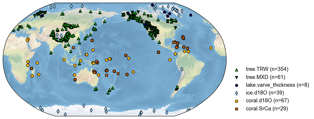
We may also plot map along with the count of the records:
[6]:
fig, ax = pdb.plot(plot_count=True)
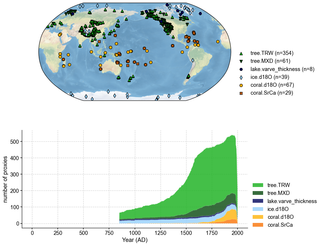
Since the dataset starts from 850 AD, we may adjust the x-axis utilizing the matplotlib methods:
[7]:
fig, ax = pdb.plot(plot_count=True)
ax['count'].set_xlim(800, 2000)
[7]:
(800.0, 2000.0)
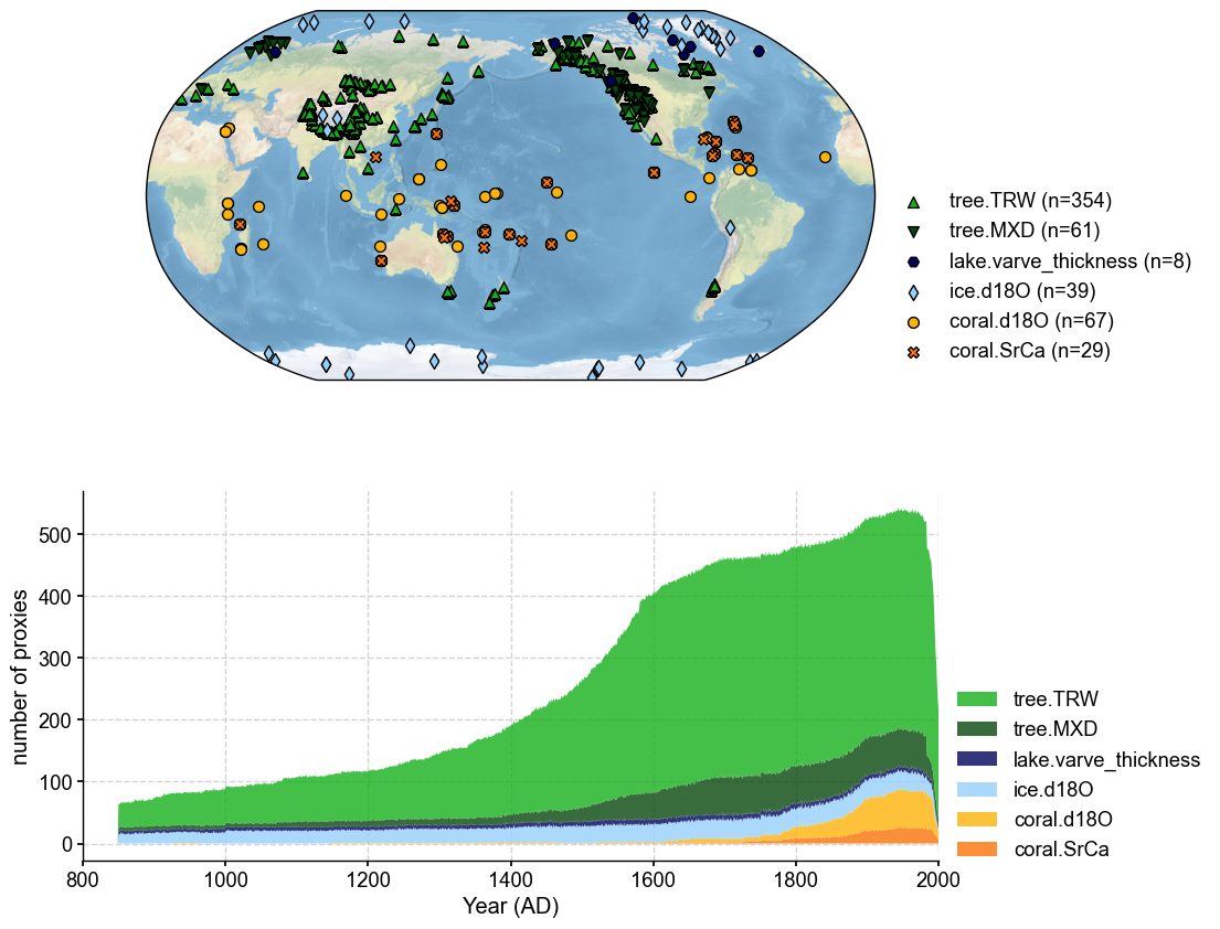
Access and visualize a specific record#
A specific record can be accessed by its proxy ID:
[8]:
pobj = pdb['NAm_001']
pobj
[8]:
<cfr.proxy.ProxyRecord at 0x2be7b3730>
This returned object is defined by cfr.ProxyRecord, which comes with several attributes such as:
time: the time axis
value: the value axis
lat: the latitude of the site
lon: the longitude of the site
(… other metadata)
For instance, to access the record series:
[9]:
print('time axis:', pobj.time)
print('value axis:', pobj.value)
time axis: [ 850.  851.  852. ... 2000. 2001. 2002.]
value axis: [1.06636798 0.86741749 0.87185387 ... 0.81825943 0.58718452 0.85097093]
Now that we have the cfr.ProxyRecord object, we can easily visualize the record utilizing the .plot() method:
[10]:
fig, ax = pobj.plot()
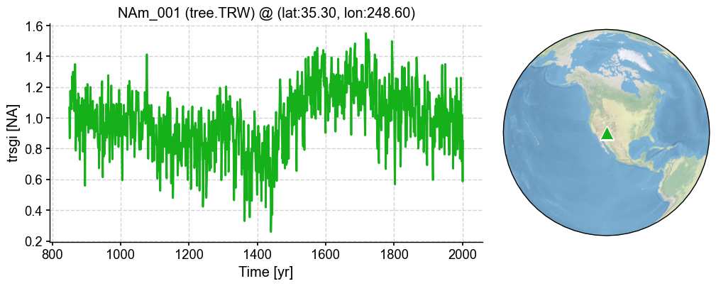
We may slice the record to zoom in and out. For instance, let us check the instrumental period:
[11]:
fig, ax = pobj.slice([1850, 2000]).plot()

We may also slice with a shortcut using strings of years:
[12]:
fig, ax = pobj['1850':'2000'].plot()
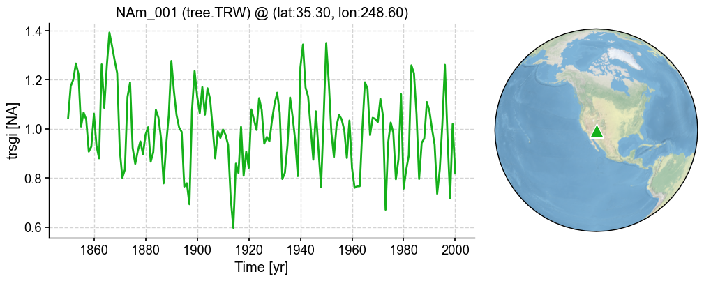
This shortcut also supports time step. For instance, to display the data points every 10 years between 1850 AD and 2000 AD:
[13]:
fig, ax = pobj['1850':'2000':'10'].plot(marker='o')
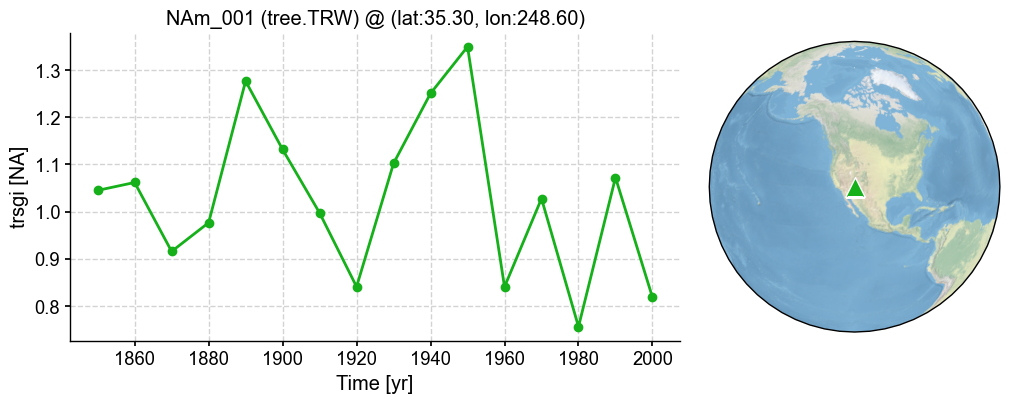
Check the proxy IDs on an interactive map#
One may ask “How do I know the proxy IDs?”
A cfr.ProxyDatabase object also comes with a .plotly() method that can help us check proxy IDs on an interactive map. It will display an interactive map, and by hovering the mouse over each site marker, one may check the metadata of a specific site, including:
pid (proxy ID)
ptype
lat
lon
[14]:
pdb.plotly()
Data type cannot be displayed: application/vnd.plotly.v1+json