Input/Output#
In this section, we illustrate how to input and output gridded climate data with cfr.
cfr provides a useful class called ClimateField to handle gridded climate data. It is essentially a wrapper of a xarray.DataArray, but with additional analysis and visualization functionalities added on.
Essentially, cfr supports below conversions:
a netCDF file <=>
cfr.ClimateFieldxarray.DataArray<=>cfr.ClimateFieldnumpy.ndarray<=>cfr.ClimateField
In addition, cfr supports remote loading of hosted gridded climate data in netCDF.
Required data to complete this tutorial:
GISTEMP surface temperature: gistemp1200_GHCNv4_ERSSTv5.nc
HadCRUTv5 surface temperature: HadCRUT.5.0.1.0.anomalies.ensemble_mean.nc
[1]:
%load_ext autoreload
%autoreload 2

import cfr
print(cfr.__version__)
import os
import xarray as xr
a netCDF file => cfr.ClimateField#
A simplest case is that the netCDF file contains only one variable with standard names for time, latitude, and longitude: time, lat, lon. In this case, we just create a cfr.ClimateField object and call its .load_nc() method with a path to the netCDF file as the argument.
Sometimes, however, the netCDF file comes with multiple variables, in which case we need to specify the variable name via the vn argument:
[2]:
dirpath = './data'
fd = cfr.ClimateField().load_nc(
    os.path.join(dirpath, 'gistemp1200_GHCNv4_ERSSTv5.nc'),  # path to the netCDF file
    vn='tempanomaly',  # specify the name of the variable to load
)
fd.da  # check the loaded `xarray.DataArray`
[2]:
<xarray.DataArray 'tempanomaly' (time: 1718, lat: 90, lon: 180)>
[27831600 values with dtype=float32]
Coordinates:
  * lat      (lat) float32 -89.0 -87.0 -85.0 -83.0 -81.0 ... 83.0 85.0 87.0 89.0
  * lon      (lon) float32 1.0 3.0 5.0 7.0 9.0 ... 351.0 353.0 355.0 357.0 359.0
  * time     (time) datetime64[ns] 1880-01-15 1880-02-15 ... 2023-02-15
Attributes:
    long_name:     Surface temperature anomaly
    units:         K
cell_methods: time: meanIf the netCDF file names the latitude and longitude dimensions with other differently, we will also need to speicify them. For instance, below we are trying to load the HadCRUT dataset, which have different names for the coordinates:
[3]:
ds = xr.open_dataset(os.path.join(dirpath, 'HadCRUT.5.0.1.0.analysis.anomalies.ensemble_mean.nc'))
ds
[3]:
<xarray.Dataset>
Dimensions:           (time: 2076, latitude: 36, longitude: 72, bnds: 2)
Coordinates:
  * time              (time) datetime64[ns] 1850-01-16T12:00:00 ... 2022-12-1...
  * latitude          (latitude) float64 -87.5 -82.5 -77.5 ... 77.5 82.5 87.5
  * longitude         (longitude) float64 -177.5 -172.5 -167.5 ... 172.5 177.5
    realization       int64 ...
Dimensions without coordinates: bnds
Data variables:
    tas_mean          (time, latitude, longitude) float64 ...
    time_bnds         (time, bnds) datetime64[ns] ...
    latitude_bnds     (latitude, bnds) float64 ...
    longitude_bnds    (longitude, bnds) float64 ...
    realization_bnds  (bnds) int64 ...
Attributes:
    comment:      2m air temperature over land blended with sea water tempera...
    history:      Data set built at: 2023-01-10T22:32:59+00:00
    institution:  Met Office Hadley Centre / Climatic Research Unit, Universi...
    licence:      HadCRUT5 is licensed under the Open Government Licence v3.0...
    reference:    C. P. Morice, J. J. Kennedy, N. A. Rayner, J. P. Winn, E. H...
    source:       CRUTEM.5.0.1.0 HadSST.4.0.0.0
    title:        HadCRUT.5.0.1.0 blended land air temperature and sea-surfac...
    version:      HadCRUT.5.0.1.0
Conventions: CF-1.7We specify the lon_name and lat_name in the arguments so that the .load_nc() method can load the data correctly. time_name may be also specified if its named differently in the netCDF file. Once loaded, those coordinates will be renamed to the standard time, lat, and lon.
[4]:
dirpath = './data'
fd = cfr.ClimateField().load_nc(
    os.path.join(dirpath, 'HadCRUT.5.0.1.0.analysis.anomalies.ensemble_mean.nc'),
    time_name='time',       # specify the name of the time dimension
    lon_name='longitude',   # specify the name of the lontitude dimension
    lat_name='latitude',    # specify the name of the latitude dimension
    vn='tas_mean',          # specify the name of the variable to load
)
fd.da  # check the loaded `xarray.DataArray`
[4]:
<xarray.DataArray 'tas_mean' (time: 2076, lat: 36, lon: 72)>
[5380992 values with dtype=float64]
Coordinates:
  * time         (time) datetime64[ns] 1850-01-16T12:00:00 ... 2022-12-16T12:...
  * lat          (lat) float64 -87.5 -82.5 -77.5 -72.5 ... 72.5 77.5 82.5 87.5
  * lon          (lon) float64 2.5 7.5 12.5 17.5 ... 342.5 347.5 352.5 357.5
    realization  int64 ...
Attributes:
    long_name:     blended air_temperature_anomaly over land with sea_water_t...
    units:         K
cell_methods: area: mean (interval: 5.0 degrees_north 5.0 degrees_east) ...cfr.ClimateField => a netCDF file#
A cfr.ClimateField can be output to a netCDF file easily with the .to_nc() method:
[5]:
fd.to_nc('./data/fd.nc')
ClimateField.da["tas_mean"] saved to: ./data/fd.nc
Now let’s check if the saved netCDF file looks fine:
[6]:
da = xr.open_dataarray('./data/fd.nc')
da
[6]:
<xarray.DataArray 'tas_mean' (time: 2076, lat: 36, lon: 72)>
[5380992 values with dtype=float64]
Coordinates:
  * time         (time) datetime64[ns] 1850-01-16T12:00:00 ... 2022-12-16T12:...
  * lat          (lat) float64 -87.5 -82.5 -77.5 -72.5 ... 72.5 77.5 82.5 87.5
  * lon          (lon) float64 2.5 7.5 12.5 17.5 ... 342.5 347.5 352.5 357.5
    realization  int64 ...
Attributes:
    long_name:     blended air_temperature_anomaly over land with sea_water_t...
    units:         K
    cell_methods:  area: mean (interval: 5.0 degrees_north 5.0 degrees_east) ...
xarray.DataArray => cfr.ClimateField#
Sometimes, we will load a xarray.DataArray first, after which we may convert it to a cfr.ClimateField with the .from_da() method:
[7]:
fd = cfr.ClimateField(da)
fd.da
[7]:
<xarray.DataArray 'tas_mean' (time: 2076, lat: 36, lon: 72)>
[5380992 values with dtype=float64]
Coordinates:
  * time         (time) datetime64[ns] 1850-01-16T12:00:00 ... 2022-12-16T12:...
  * lat          (lat) float64 -87.5 -82.5 -77.5 -72.5 ... 72.5 77.5 82.5 87.5
  * lon          (lon) float64 2.5 7.5 12.5 17.5 ... 342.5 347.5 352.5 357.5
    realization  int64 ...
Attributes:
    long_name:     blended air_temperature_anomaly over land with sea_water_t...
    units:         K
cell_methods: area: mean (interval: 5.0 degrees_north 5.0 degrees_east) ...cfr.ClimateField => xarray.DataArray#
The convertion from a cfr.ClimateField to a xarray.DataArray is trivial: simply access the .da attribute:
[8]:
da = fd.da
da
[8]:
<xarray.DataArray 'tas_mean' (time: 2076, lat: 36, lon: 72)>
[5380992 values with dtype=float64]
Coordinates:
  * time         (time) datetime64[ns] 1850-01-16T12:00:00 ... 2022-12-16T12:...
  * lat          (lat) float64 -87.5 -82.5 -77.5 -72.5 ... 72.5 77.5 82.5 87.5
  * lon          (lon) float64 2.5 7.5 12.5 17.5 ... 342.5 347.5 352.5 357.5
    realization  int64 ...
Attributes:
    long_name:     blended air_temperature_anomaly over land with sea_water_t...
    units:         K
cell_methods: area: mean (interval: 5.0 degrees_north 5.0 degrees_east) ...numpy.ndarray => cfr.ClimateField#
We may also convert a collection of numpy.ndarrays to a cfr.ClimateField:
[9]:
time = da.time.values
lat = da.lat.values
lon = da.lon.values
value = da.values
print(type(time), type(lat), type(lon), type(value))
print(value.shape)
<class 'numpy.ndarray'> <class 'numpy.ndarray'> <class 'numpy.ndarray'> <class 'numpy.ndarray'>
(2076, 36, 72)
[10]:
fd = cfr.ClimateField().from_np(
    time, lat, lon, value,
)
fd.da
[10]:
<xarray.DataArray (time: 2076, lat: 36, lon: 72)>
array([[[       nan,        nan,        nan, ...,        nan,
                nan,        nan],
        [       nan,        nan,        nan, ...,        nan,
                nan,        nan],
        [       nan,        nan,        nan, ...,        nan,
                nan,        nan],
        ...,
        [-0.7109375, -0.7421875, -0.8046875, ..., -0.6875   ,
         -0.6875   , -0.6875   ],
        [-0.890625 , -0.921875 , -0.9609375, ...,        nan,
                nan, -0.875    ],
        [       nan,        nan,        nan, ...,        nan,
                nan,        nan]],

       [[       nan,        nan,        nan, ...,        nan,
                nan,        nan],
        [       nan,        nan,        nan, ...,        nan,
                nan,        nan],
        [       nan,        nan,        nan, ...,        nan,
                nan,        nan],
...
        [ 2.6875   ,  2.1328125,  2.984375 , ...,  4.75     ,
          4.796875 ,  4.0859375],
        [ 4.4296875,  4.53125  ,  4.5      , ...,  4.0078125,
          4.171875 ,  4.3125   ],
        [ 3.6015625,  3.640625 ,  3.671875 , ...,  3.484375 ,
          3.5234375,  3.5703125]],

       [[-1.0859375, -1.109375 , -1.125    , ..., -1.0234375,
         -1.046875 , -1.0703125],
        [-1.0546875, -1.0859375, -1.1171875, ..., -0.953125 ,
         -0.984375 , -1.0234375],
        [-0.8359375, -0.8828125, -0.9453125, ..., -0.7265625,
         -0.7578125, -0.796875 ],
        ...,
        [ 1.3203125,  1.2578125,  2.09375  , ...,  1.90625  ,
          1.875    ,  1.6484375],
        [ 3.6953125,  3.7890625,  3.578125 , ...,  3.5390625,
          3.5703125,  3.625    ],
        [ 4.4921875,  4.515625 ,  4.5390625, ...,  4.421875 ,
          4.4453125,  4.46875  ]]])
Coordinates:
  * time     (time) datetime64[ns] 1850-01-16T12:00:00 ... 2022-12-16T12:00:00
  * lat      (lat) float64 -87.5 -82.5 -77.5 -72.5 -67.5 ... 72.5 77.5 82.5 87.5
* lon (lon) float64 2.5 7.5 12.5 17.5 22.5 ... 342.5 347.5 352.5 357.5cfr.ClimateField => numpy.ndarray#
The conversion from a cfr.ClimateField to a collection of numpy.ndarrays is trivial:
[11]:
time = fd.da.time.values
lat = fd.da.lat.values
lon = fd.da.lon.values
value = fd.da.values
print(type(time), type(lat), type(lon), type(value))
print(value.shape)
<class 'numpy.ndarray'> <class 'numpy.ndarray'> <class 'numpy.ndarray'> <class 'numpy.ndarray'>
(2076, 36, 72)
Remote loading gridded climate data#
cfr supports remote loading of hosted gridded climate data in netCDF files, currently including iCESM past1000 and past1000historical.
By calling the .fetch() method of ClimateField without any arguments, a list of supported simulation names will be listed:
[4]:
fd = cfr.ClimateField().fetch()
>>> Choose one from the supported entries: ['iCESM_past1000historical/tas', 'iCESM_past1000historical/pr']
Remote loading iCESM simulations#
The target netCDF file will be downloaded to the relative directory ./data if not existed (skipped if existed), after which a ClimateField() will be built with that netCDF file.
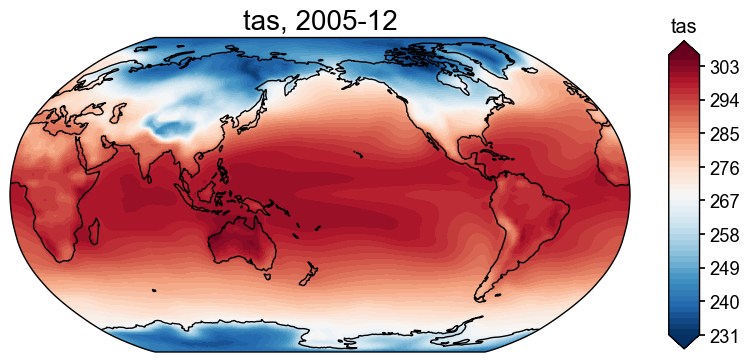
[6]:
# the case when the file exists already
fd = cfr.ClimateField().fetch('iCESM_past1000historical/tas')
fig, ax = fd[-1].plot()
>>> The target file seems existed at: ./data/tas_sfc_Amon_iCESM_past1000historical_085001-200512.nc . Loading from it instead of downloading ...
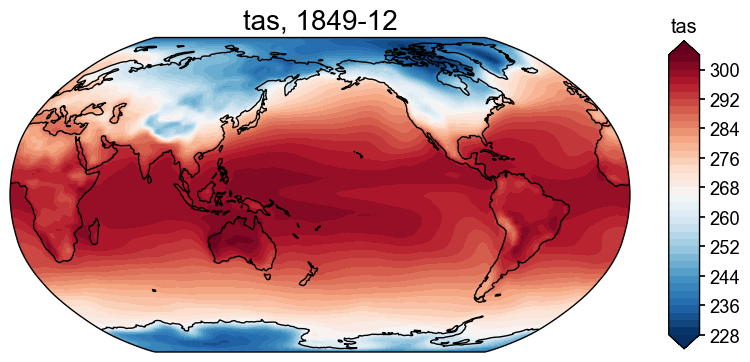
[10]:
# the case when the file doesn't exist
fd = cfr.ClimateField().fetch('iCESM_past1000/tas')
fig, ax = fd[-1].plot()
Fetching data: 100%|██████████| 633M/633M [00:09<00:00, 66.7MiB/s]
>>> Downloaded file saved at: ./data/tas_sfc_Amon_iCESM_past1000_085001-184912.nc .
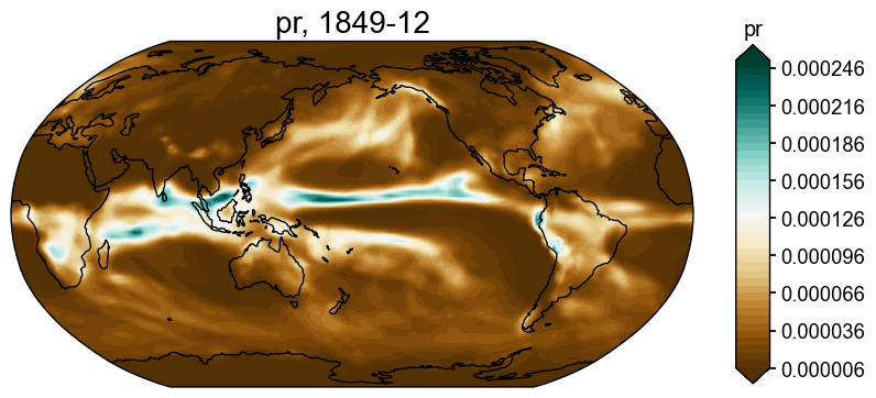
We may also specify a URL to fetch arbitray netCDF files:
[12]:
fd = cfr.ClimateField().fetch('https://atmos.washington.edu/~rtardif/LMR/prior/pr_sfc_Amon_iCESM_past1000_085001-184912.nc')
fig, ax = fd[-1].plot()
Fetching data: 100%|██████████| 633M/633M [00:10<00:00, 66.2MiB/s]
>>> Downloaded file saved at: ./data/pr_sfc_Amon_iCESM_past1000_085001-184912.nc .
[ ]: