Basic Operations

Basic Operations#

In this section, we introduce the basic operations of a cfr.ClimateField.

Required data to complete this tutorial:

GISTEMP surface temperature: gistemp1200_GHCNv4_ERSSTv5.nc

Due to the new data fetching feature, the above datasets are not required to be downloaded manually.

[1]:

%load_ext autoreload
%autoreload 2

import cfr
print(cfr.__version__)
import numpy as np

2024.12.4

Plot a field map at a time point#

[30]:

fig, ax = fd['1990-11'].plot()

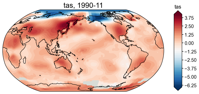
../_images/notebooks_climate-ops_18_0.png

The default colorbar is not zero-centered. We may adjust as below:

[31]:

fig, ax = fd['1990-11'].plot(
    levels=np.linspace(-5, 5, 21),       # set levels for the colors
    cbar_labels=np.linspace(-5, 5, 11),  # set the labels for the bar
)

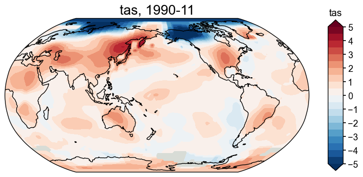
../_images/notebooks_climate-ops_20_0.png

Get the anomaly field#

We may call the .get_anom() method, specifying a reference period, to calculate the anomaly field:

[32]:

fd_anom = fd.get_anom(ref_period=(1951, 2000))
fig, ax = fd_anom['1990-11'].plot(
    levels=np.linspace(-5, 5, 21),       # set levels for the colors
    cbar_labels=np.linspace(-5, 5, 11),  # set the labels for the bar
    extend='both',                       # extend the bar
)

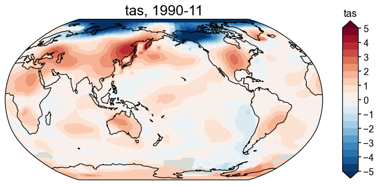
../_images/notebooks_climate-ops_22_0.png

Center the field#

Similar to calculating the anomaly, sometimes we just want to center the values of a field against a reference period. With a cfr.ClimateField, we may call the .center() method to achieve that, again speciying a reference period:

[33]:

fd_center = fd.center(ref_period=(1951, 2000))
fig, ax = fd_center['1990-11'].plot(
    levels=np.linspace(-5, 5, 21),       # set levels for the colors
    cbar_labels=np.linspace(-5, 5, 11),  # set the labels for the bar
    extend='both',                       # extend the bar
)

../_images/notebooks_climate-ops_24_0.png

Calculate the weighted mean of a sptial area#

Lots of climatic indices require to calculate the weighted mean of a spatial area, e.g., the global mean surface temperature (GMST), NINO3.4, etc.

With a cfr.ClimateField, we may call the .geo_mean() method to calculate that quantity, again specifying the arguments lat_min, lat_max, lon_min, lon_max.

[39]:

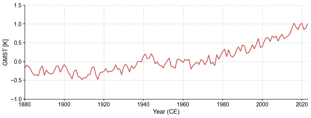
gmst = fd.annualize().geo_mean()  # by default, the area is global
fig, ax = gmst.plot(ylabel='GMST [K]', linewidth=2, ylim=(-1, 1.5))

../_images/notebooks_climate-ops_34_0.png

[40]:

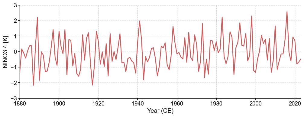
nino34 = fd.annualize(months=[12, 1, 2]).geo_mean(
    lat_min=-5, lat_max=5,
    lon_min=np.mod(-170, 360), lon_max=np.mod(-120, 360)
)
fig, ax = nino34.plot(ylabel='NINO3.4 [K]', linewidth=2, ylim=(-3, 3))

../_images/notebooks_climate-ops_35_0.png

Validate a field against another#

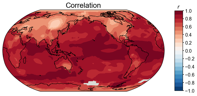
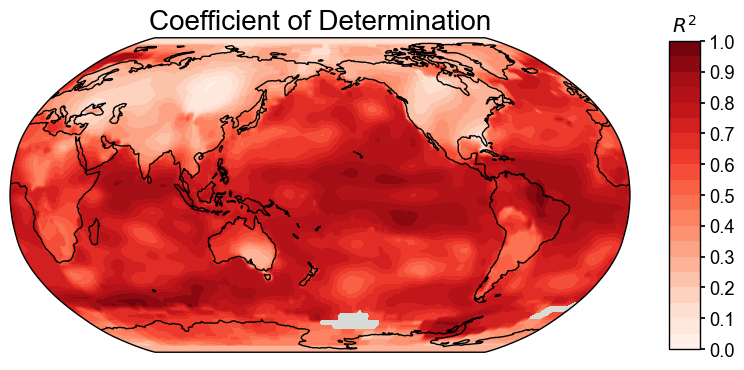
We may compare two cfr.ClimateFields by calling the .compare() method. Here as an example, we compare the calendar year annualized field with the JJA annualized field, with three different metrics:

[15]:

for stat in ['corr', 'R2', 'CE']:
    valid_fd = fd['1880':'2000'].annualize().compare(
        fd['1880':'2000'].annualize(months=[6, 7, 8]), stat=stat)
    fig, ax = valid_fd.plot()

../_images/notebooks_climate-ops_37_0.png

../_images/notebooks_climate-ops_37_1.png

../_images/notebooks_climate-ops_37_2.png

[ ]:

Basic Operations

Contents

Basic Operations#

Load the test netCDF file as a `ClimateField`#

Time slicing#

Rename the variable#

Plot a field map at a time point#

Get the anomaly field#

Center the field#

Annualize/Seasonalize a `ClimateField`#

Regrid a `ClimateField`#

Crop a `cfr.ClimateField`#

Calculate the weighted mean of a sptial area#

Validate a field against another#

Basic Operations

Contents

Basic Operations#

Load the test netCDF file as a ClimateField#

Time slicing#

Rename the variable#

Plot a field map at a time point#

Get the anomaly field#

Center the field#

Annualize/Seasonalize a ClimateField#

Regrid a ClimateField#

Crop a cfr.ClimateField#

Calculate the weighted mean of a sptial area#

Validate a field against another#

Load the test netCDF file as a `ClimateField`#

Annualize/Seasonalize a `ClimateField`#

Regrid a `ClimateField`#

Crop a `cfr.ClimateField`#